
Dive into the world of image segmentation, where pixels become storytellers. On this journey, I will uncover the secret of how simple pixels become meaningful predictions. Join me and explore the art and science of image decoding. Get ready for a fascinating adventure that demystifies the magic behind images. Let’s go on this enlightening journey together!
- Image Classification & Image Segmentation
- Image Segmentation Experiment: Insights from my Capstone Project
- Navigating the Dataset Challenges
- Network Architectures
- Tweaking input data and optimizing model and runtime
- Final model
- Exploring further improvement ideas
Image Classification & Image Segmentation
Welcome to the exciting area of image segmentation! In the ML Zoomcamp course, masterfully crafted by Alexey Grigorev (DataTalk.club), we delved into the captivating world of image classification. Now, while both image classification and segmentation share a common ground in dealing with images, the neural network architecture orchestrating their magic differs significantly. This disparity is driven by the distinct nature of their prediction goals.
In the domain of image classification, our neural network aspires to predict a singular label for the entire image. Whether it’s about the distinction between a cat, a dog, a car, or any other label, the focus is on classifying the image as a whole. However, when it comes to image segmentation, the game changes dramatically. Here, our neural network aims to predict a class for every individual pixel in the image.
Let’s envision this with animal images for clarity. In image segmentation, the goal is not merely to identify a cat in the image but to carefully separate the cat from its background. Imagine our model examining each pixel, making decisions like “cat” or “no cat.” And just to spice things up, we can have more than one class, leading us into the fascinating area of multi-class image segmentation problems.
In both scenarios, the output of our neural network is not a conventional class label. Instead, it produces an entire image, mirroring the pixel spacing of the input image. Achieving this goal requires a special architecture of neural networks that paves the way for exciting research into the complexities of image segmentation. So get ready to unleash the secrets behind the pixels and discover the fascinating world of segmentation!
Image Segmentation Experiment: Insights from my Capstone Project
As I entered the challenging terrain of my Capstone Project 2, I decided to take the road less traveled – image segmentation. Leaving the familiar domains of regression and image classification covered in our course, I had no idea what a brave adventure was waiting for me.
For this venture, I delved into the LandCover.ai (Land Cover from Aerial Imagery) dataset, a resource for automatic mapping of buildings, woodlands, water, and roads from aerial imagery. The package includes: 33 orthophotos (RGB) with a resolution of 25 cm per pixel (~9000×9500 px), accompanied by 8 orthophotos (RGB) at a slightly lower 50 cm per pixel resolution (~4200×4700 px). This dataset, covering an area of 216.27 km² of Poland, presented both a challenge and an opportunity.
You can find some more information especially about the license information on the web link mentioned before. The data set recommends the use of 512×512 pixel fields, but I quickly realized the limits of my local computer. Nevertheless, this problem barely affected my enthusiasm.
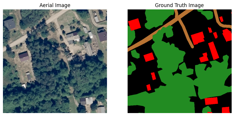
To give you an idea of what’s in the data, let’s look at a sample aerial image together with the corresponding ground truth mask. Each pixel of the image on the right is associated with an aerial image pixel on the left and indicates class membership. Each of the four classes has a special color tone:
- woodlands – green
- buildings – red
- water – blue
- roads – light brown
- unlabeled – black
Navigating the Dataset Challenges
The image above illustrates the challenges hidden in the LandCover.ai dataset. In particular, the presence of the many black pixels presents a significant obstacle. These pixels belong to a class for which the model is kept from further differentiation. This group includes fields, wetlands, bare ground, rocks and more. This mixing of feature classes is a potential pitfall that requires our attention. Maintaining a delicate balance is crucial to ensure that the number of unlabeled pixels remains relatively low. An excess could mislead the model and tempt it to unintentionally learn this unwanted feature class.
An observant eye will also recognize the insufficiencies in the ground truth (GT) mask. It is no secret that the best possible GT mask is the key to an optimal model performance. The mantra here is clear: the better the GT, the better the model is able to navigate unfamiliar terrain.
Undaunted by these challenges, I began my journey with a simple model, only to realize that my machine crashed under the pressure. So I had to look at making the big patches more manageable. Join me on my journey through the maze of challenges to a usable model.
def model(input_size=(512, 512, 3), num_classes=5):
    inputs = keras.Input(input_size)

    # Encoder
    conv1 = layers.Conv2D(64, 3, activation="relu", padding="same")(inputs)
    conv1 = layers.Conv2D(64, 3, activation="relu", padding="same")(conv1)
    pool1 = layers.MaxPooling2D(pool_size=(2, 2))(conv1)

    # Decoder
    conv2 = layers.Conv2D(128, 3, activation="relu", padding="same")(pool1)
    conv2 = layers.Conv2D(128, 3, activation="relu", padding="same")(conv2)
    up1 = layers.UpSampling2D((2, 2))(conv2)

    # Output layer with softmax activation for multi-class classification
    outputs = layers.Conv2D(num_classes, 1, activation="softmax")(up1)

    model = keras.Model(inputs, outputs)
    return model
Challenges – Running a Simple Network
In my quest to master the challenges of image segmentation, I started with a simple neural network. As mentioned earlier, the first attempt with 512×512 image patches failed. The second attempt with 256×256 image fields was more successful.
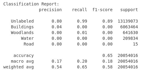
After completing 10 epochs of training, the final results showed a mixed picture:
loss: 0.4100 – accuracy: 0.8518 – val_loss: 0.4925 – val_accuracy: 0.8212
At first glance, the validation accuracy seemed acceptable for a developing model. But appearances are deceptive. Behind this seemingly positive result lies the harsh reality of the enormous number of unlabeled pixels in this dataset. These unlabeled areas pose a major challenge for the model and make the learning process considerably more difficult. Unfortunately, this model is useless. Let’s see whether we can improve the situation.

Challenges – Imbalanced Dataset
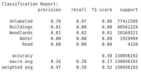
In my journey towards a usable image segmentation model, I have focused my attention on one key aspect – the class distribution in my dataset. The results of this investigation are both illuminating and worrying, and paint a clear picture of the complexity of the dataset.
Take a look at the class distribution below:
- “Unlabeled” class: This undesirable class dominates the landscape and is almost twice as prevalent as the second largest class, “Woodlands”.
- “Woodlands” class: The second largest class accounts for almost a third of all pixels.
- “Water” class: This class has a share of just under 6%
Classes “Buildings” and “Roads”: These classes are strongly underrepresented and together do not even come to 3%.
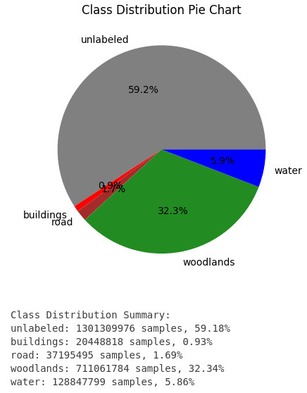
The strong imbalance in class distribution is a major challenge. The overpowering presence of the “Unlabeled” class threatens to hinder the model’s ability to recognize and learn effectively. To address this imbalance, I tried to optimize the dataset. I will go into more detail about how I did this later.
Challenges – Smaller Image patches
Another hurdle popped up as I grappled with the size of the image patches. Initial attempts with 512×512 image fields proved too taxing for my computer, so I switched to the seemingly more manageable 256×256 dimension. However, the path to resolution was not as easy as expected.
Despite the adjustment, a number of complications arose with 256×256 image fields. I had to reduce the size to 128×128. Finally, this step allowed a smoother investigation. This led me to another important decision – choosing the optimal resampling method to find the right balance between computing power and image quality.
Challenges – Resampling
As already mentioned, the selection of the ideal resampling filter is also important.
Pillow, which I used in version 10.2.0, offers six options here: NEAREST, BOX, BILINEAR, HAMMING, BICUBIC, LANCZOS (renamed from “ANTIALIAS” in former Pillow versions).
The comprehensive Pillow documentation (https://pillow.readthedocs.io/en/stable/handbook/concepts.html#concept-filters) shows that the “LANCZOS” resampling method produces the best quality. This quality comes at the expense of performance, which I considered negligible at this time.
Network Architectures
Improved Simple Model – using class weights
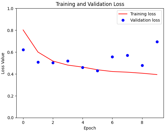
Using a resampled training dataset with a size of 128×128, I attempted to improve the capabilities of the previously described network. This time, however, the focus went beyond just accuracy tracking; I delved into the metrics of accuracy and mIoU (mean Intersection over Union). At the same time, I investigated the impact of class weights on model performance.
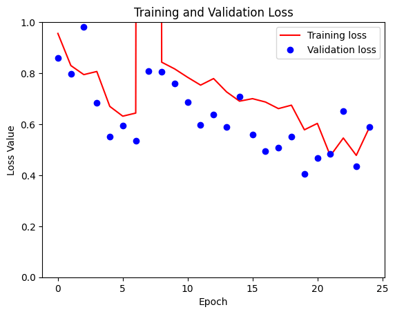
For comparison, I have shown training loss and validation loss for the model without class weights here.
From the initial summary of the class distribution, I gained a nuanced understanding of the distribution across the different classes:
Class 0: Unlabeled (59%)
Class 1: Forest areas (32%)
Class 2: Water (6%)
Class 3: Roads (2%)
Class 4: Buildings (1%)
These weights serve as guiding principles for the model and introduce a dynamic element to loss calculation. By assigning weights that reflect the class distribution, the model adapts to errors differently depending on the landcover class in which they occur. At the end an error in case of the last three classes (water, roads, and buildings) should lead to a bigger adaptation of the weights.
The configuration of class weights used in the training process was defined as follows:
class_weights = {0: .59, 1: .32, 2: .06, 3: .02, 4: .01}
...
# Train the model with class weights and checkpoint callback
model_history = model.fit(X_train, y_train,
                          epochs=epochs,
                          batch_size=batch_size,
                          validation_data=(X_val, y_val),
                          class_weight=class_weights,
                          callbacks=[checkpoint]
)
As the training progressed, the introduction of class weights had a noticeable effect. Train loss decreased remarkably and was significantly lower than its predecessor. Despite this significant decrease in training loss, validation loss reacted more cautiously and showed only a marginal change. This nuanced divergence between training and validation performance is a crucial observation.
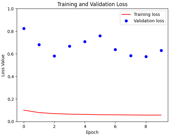
Contrary to expectations, the model with class weights unfortunately performed worse on the validation data than its simpler counterpart without these weight adjustments. The background currently remains a mystery to me and needs deeper analysis.
U-Net model
I’ve found a U-Net implementation here which I used for the next runs.
def double_conv_block(x, n_filters):
   # Conv2D then ReLU activation
   x = layers.Conv2D(n_filters, 3, padding = "same", activation = "relu", kernel_initializer = "he_normal")(x)
   # Conv2D then ReLU activation
   x = layers.Conv2D(n_filters, 3, padding = "same", activation = "relu", kernel_initializer = "he_normal")(x)
   return x

def downsample_block(x, n_filters):
   f = double_conv_block(x, n_filters)
   p = layers.MaxPool2D(2)(f)
   p = layers.Dropout(0.3)(p)
   return f, p

def upsample_block(x, conv_features, n_filters):
   # upsample
   x = layers.Conv2DTranspose(n_filters, 3, 2, padding="same")(x)
   # concatenate
   x = layers.concatenate([x, conv_features])
   # dropout
   x = layers.Dropout(0.3)(x)
   # Conv2D twice with ReLU activation
   x = double_conv_block(x, n_filters)
   return x

# Define U-Net model for 5 classes
def unet_model(input_size=(128, 128, 3), num_classes=5):
    inputs = keras.Input(input_size)

    # encoder: contracting path - downsample
    # 1 - downsample
    f1, p1 = downsample_block(inputs, 64)
    # 2 - downsample
    f2, p2 = downsample_block(p1, 128)
    # 3 - downsample
    f3, p3 = downsample_block(p2, 256)
    # 4 - downsample
    f4, p4 = downsample_block(p3, 512)
    # 5 - bottleneck
    bottleneck = double_conv_block(p4, 1024)
    # decoder: expanding path - upsample
    # 6 - upsample
    u6 = upsample_block(bottleneck, f4, 512)
    # 7 - upsample
    u7 = upsample_block(u6, f3, 256)
    # 8 - upsample
    u8 = upsample_block(u7, f2, 128)
    # 9 - upsample
    u9 = upsample_block(u8, f1, 64)
    # outputs
    outputs = layers.Conv2D(num_classes, 1, padding="same", activation = "softmax")(u9)
    # unet model with Keras Functional API
    unet_model = tf.keras.Model(inputs, outputs, name="U-Net")
    return unet_model
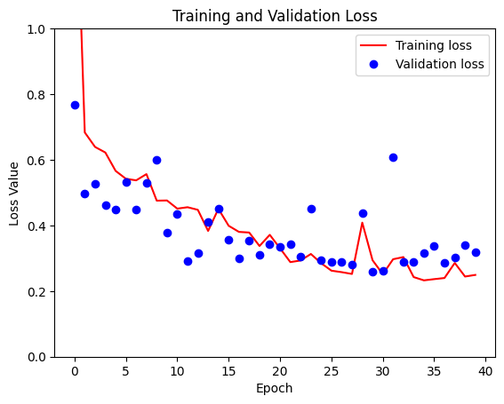
Let’s now look at the comparison between the simple U-Net scenario without weights and the U-Net model with the application of predefined class weights. The scenario without weights looks very similar to the simple model scenario. Both losses showing sub-optimal performance, but within a comparable range.

I then used the predefined class weights in the U-Net model. To my surprise, the scenario without weights mirrored the simple situation very well, showing similar losses and leaving me with dampened expectations of an improved classification report.

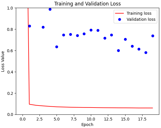
When plotting the results, a familiar pattern emerged in both experiments – the strong influence of the predefined class weights. In both the simple model and the U-Net architecture, the application of these weights only led to a significant reduction in training losses, which is actually expected evidence of adaptability.
However, the evaluation on the validation set showed a different, but unfortunately familiar, picture. Despite the noticeable effects on training loss, the positive effects of the predefined class weights in the validation set were absent for both scenarios. As intriguing as this observation may be, it led me to withdraw from including predefined class weights in my subsequent experiments.
DeepLabV3
On my way to find the optimal architecture for image segmentation, I came across DeepLabV3, a promising competitor that would complete the field. This encounter was short-lived because a perplexing challenge arose during validation. It was an anomaly where the model provided an identical prediction for any given image. This unexpected behavior was an obstacle and led to the decision to stop looking at the DeepLabV3 model for the moment.
Tweaking input data and optimizing model and runtime
I wanted to improve the situation. On the one hand training runtime was to long and the input data was not good enough. To reduce training runtime I used a resampling that transformed image patches to a more manageable size of (128×128). At the same time, I tried to improve the input quality while reducing the big share of unlabeled pixels.
I examined the effects of excluding images with different thresholds for the proportion of unlabeled pixels. The resulting table showed significant changes in the composition of the dataset and in the class distribution.
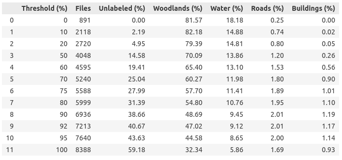
After careful consideration, I decided to use a threshold of 80% (later I also used 20% as a threshold). This decision led to a significant reduction of the training dataset from 8,388 to 5,999 images and at the same time to a reduction of the proportion of unlabeled pixels from 59% to 31%. This step not only improved the class balance, but also made the dataset more manageable, promising a potential reduction in training time per epoch.
On the basis of image patches of size (128 x 128) I did some tuning. I used different metrics (binary cross entropy, categorical cross entropy, MeanIoU, MSE, TP, FP, TN, FN, accuracy, precision, recall, AUC)…
METRICS = [
keras.metrics.BinaryCrossentropy(name=’cross entropy’),
keras.metrics.CategoricalCrossentropy(name=’cat_cross_entropy’),
keras.metrics.MeanIoU(name=’mIoU’, num_classes=num_classes),
keras.metrics.MeanSquaredError(name=’Brier score’),
keras.metrics.TruePositives(name=’tp’),
keras.metrics.FalsePositives(name=’fp’),
keras.metrics.TrueNegatives(name=’tn’),
keras.metrics.FalseNegatives(name=’fn’),
keras.metrics.BinaryAccuracy(name=’accuracy’),
keras.metrics.Precision(name=’precision’),
keras.metrics.Recall(name=’recall’),
keras.metrics.AUC(name=’auc’)
]
… and I’ve tried to increase the model performance by using dropout.
The use of callbacks was discussed in the course. There, a callback ModelCheckpoint is used to reduce the number of saved models. While using ModelCheckpoint callback, a model is only saved, if it is better than the last model saved in relation to a defined metric.
However, there is (at least) one other callback that you should pay attention to.
early_stopping = tf.keras.callbacks.EarlyStopping(
monitor=’val_prc’,
patience=10,
mode=’max’)
EarlyStopping is used to stop the training process if a defined metric (monitor=’val_prc’) has not improved after some defined epochs (patience=10). The mode indicates what is better. Here ‘max’ means the higher the better.
The potential impact of EarlyStopping is profound. Envision a training setup scheduled for 100 epochs. Without EarlyStopping, the process would inevitably traverse the full 100 epochs. However, with EarlyStopping in play, the training might conclude much earlier, say after 20 epochs, if no discernible improvement in the specified metric is observed. This integration of EarlyStopping not only saves computational resources, but also speeds up the training process and allows a more flexible approach.
Final model
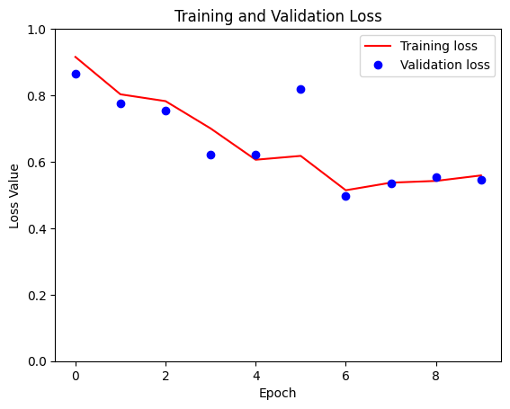
At the peak of this journey, I reached a significant milestone – successfully training different models tailored to different patch sizes, including (128×128), (256×256) and even the most sophisticated version (512×512). As the patch size increased, the runtime per epoch also increased, ranging from a brisk 2.5 minutes for the smallest patch size to 30 minutes for the largest patch size. Given the computational limitations, the final run was limited to 10 epochs. For comparison, I have plotted the loss plots for all three patch sizes.
The core of the neural network architecture used in this project is based on a basic implementation, but slightly adapted to the specific requirements of this task.
def double_conv_block(x, n_filters):
   # Conv2D then ReLU activation
   x = layers.Conv2D(n_filters, 3, padding = "same", activation = "relu", kernel_initializer = "he_normal")(x)
   # Conv2D then ReLU activation
   x = layers.Conv2D(n_filters, 3, padding = "same", activation = "relu", kernel_initializer = "he_normal")(x)
   return x

def downsample_block(x, n_filters):
   f = double_conv_block(x, n_filters)
   p = layers.MaxPool2D(2)(f)
   p = layers.Dropout(0.5)(p)
   return f, p

def upsample_block(x, conv_features, n_filters):
   # upsample
   x = layers.Conv2DTranspose(n_filters, 3, 2, padding="same")(x)
   # concatenate
   x = layers.concatenate([x, conv_features])
   # dropout
   x = layers.Dropout(0.5)(x)
   # Conv2D twice with ReLU activation
   x = double_conv_block(x, n_filters)
   return x

# Define U-Net model for 5 classes
def unet_model(input_size=(128, 128, 3), num_classes=5):
    inputs = keras.Input(input_size)

    # encoder: contracting path - downsample
    # 1 - downsample
    f1, p1 = downsample_block(inputs, 64)
    # 2 - downsample
    f2, p2 = downsample_block(p1, 128)
    # 3 - downsample
    f3, p3 = downsample_block(p2, 256)
    # 4 - downsample
    f4, p4 = downsample_block(p3, 512)
    # 5 - bottleneck
    bottleneck = double_conv_block(p4, 1024)
    # decoder: expanding path - upsample
    # 6 - upsample
    u6 = upsample_block(bottleneck, f4, 512)
    # 7 - upsample
    u7 = upsample_block(u6, f3, 256)
    # 8 - upsample
    u8 = upsample_block(u7, f2, 128)
    # 9 - upsample
    u9 = upsample_block(u8, f1, 64)
    # outputs
    outputs = layers.Conv2D(num_classes, 1, padding="same", activation = "softmax")(u9)
    # unet model with Keras Functional API
    unet_model = tf.keras.Model(inputs, outputs, name="U-Net")
    return unet_model
The next code snippet shows the use of both callbacks as well as the consideration of several metrics during training. The boolean variable USE_CLASS_WEIGTHS serves as a switch that allows training with predefined class weights and training without. I have not yet been able to derive any added value from this, but perhaps I was just overlooking the correct configuration.
# Initialize and compile the model
    model_unet = unet_model(input_size=INPUT_SIZE, num_classes=NUM_CLASSES)
    model_unet.compile(optimizer="adam", loss="categorical_crossentropy", metrics=METRICS)

    early_stopping = tf.keras.callbacks.EarlyStopping(
        monitor='val_prc',
        verbose=1,
        patience=10,
        mode='max',
        restore_best_weights=True)

    # Define the ModelCheckpoint callback
    checkpoint = ModelCheckpoint(
        'model_unet_{epoch:02d}_{val_accuracy:.3f}.keras',
        monitor='val_accuracy',     # Monitor validation accuracy
        save_best_only=True,
        save_weights_only=False,    # Save entire model
        mode='max',                 # Save the model with the highest validation accuracy
        verbose=1
    )

    # Train the model with class weights and checkpoint callbacks for model saving and early stopping
    if(USE_CLASS_WEIGTHS):
        model_unet.fit(
            X_train, y_train,
            epochs=TRAIN_EPOCHS,
            batch_size=BATCH_SIZE,
            validation_data=(X_val, y_val),
            class_weight=CLASS_WEIGHTS,
            callbacks=[checkpoint, early_stopping]
        )
    else:
        # Train the model without class weights but with checkpoint callbacks for model saving and early stopping
        model_unet_history = model_unet.fit(
            X_train, y_train,
            epochs=TRAIN_EPOCHS,
            batch_size=BATCH_SIZE,
            validation_data=(X_val, y_val),
            callbacks=[checkpoint, early_stopping]
        )
You can find the code in my repository on GitHub.
Exploring further improvement ideas
In the final notes on the realization of this prototype, it is important to acknowledge the limitations that the ticking clock imposed on the scope of this project. The time available for exploration was limited, forcing me to make decisions and push the boundaries of depth in certain areas. This prototype invites the interested reader to give free rein to their creativity and make further improvements.
Try other architectures
The landscape of image segmentation is immense, and this project only scratches the surface. Countless other architectures are waiting to be tested, each with their own promise and potential. You can look into more complicated neural networks, experiment with the number of input layers, or even explore the use of black and white images as an alternative to RGB.
Better model tuning
The performance of the model can be further refined by changing various parameters, e.g. the choice of optimizer, the loss function, adding more inner layers to the network or increasing the number of training epochs. Experiment with different configurations to find the nuances that lead to optimal results.
Improve pre- and post-processing
Improved pre-processing techniques can also be explored to provide better inputs to the model to improve performance. Post-processing the output images is another way to improve quality and refine the final segmentation results.
Proper use of “class_weights”
The model parameter “class_weight” offers unused potential. Careful exploration of its proper use, possibly incorporating dynamic adjustments during training, could lead to more refined and balanced results.
