
Adding more layers
It’s possible to add more inner layers after the vector representation. Previously we had one inner layer before outputting the prediction. This layer does some intermediate processing of the vector representation. These inner layers make the neural network more powerful.
Adding one inner dense layer
Usually adding one or two additional layers help and this is something we want to test. This layer we want to add is between the previous input and output. Let’s add one inner dense layer with size of 100. For this new layer we need an activation. In neural networks each layer should have some transformation in order to achieve better performance. We will use here “relu” as activation function.
Activation functions:
- SIGMOID (mostly used for output)
- SOFTMAX (mostly used for output)
- RELU (mostly used for intermediate layers, default value)
- …
For more information on that topic look check again the mentioned CS231n course (Neural Networks Part 1: Setting up the Architecture -> Commonly used activation functions)
To see how much gpu is utilized you can open a terminal right from Jupyter notebook and type “nvidia-smi”
Experimenting with different sizes of inner layer
def make_model(learning_rate=0.01, size_inner=100):
    base_model = Xception(
        weights='imagenet',
        include_top=False,
        input_shape=(150, 150, 3)
    )

    base_model.trainable = False

    #########################################

    inputs = keras.Input(shape=(150, 150, 3))
    base = base_model(inputs, training=False)
    vectors = keras.layers.GlobalAveragePooling2D()(base)

    inner = keras.layers.Dense(size_inner, activation='relu')(vectors)

    outputs = keras.layers.Dense(10)(inner)

    model = keras.Model(inputs, outputs)

    #########################################

    optimizer = keras.optimizers.Adam(learning_rate=learning_rate)
    loss = keras.losses.CategoricalCrossentropy(from_logits=True)

    model.compile(
        optimizer=optimizer,
        loss=loss,
        metrics=['accuracy']
    )

    return model
learning_rate = 0.001

scores = {}

for size in [10, 100, 1000]:
    print(size)

    model = make_model(learning_rate=learning_rate, size_inner=size)
    history = model.fit(train_ds, epochs=10, validation_data=val_ds)
    scores[size] = history.history

    print()
    print()

# Output:
# 10
# Epoch 1/10
# 96/96 [==============================] - 129s 1s/step - loss: 1.5733 - accuracy: 0.5059 - val_loss: 1.1653 - val_accuracy: 0.6422
# Epoch 2/10
# 96/96 [==============================] - 138s 1s/step - loss: 1.0018 - accuracy: 0.6819 - val_loss: 0.8641 - val_accuracy: 0.7302
# Epoch 3/10
# 96/96 [==============================] - 126s 1s/step - loss: 0.7346 - accuracy: 0.7578 - val_loss: 0.7169 - val_accuracy: 0.7742
# Epoch 4/10
# 96/96 [==============================] - 140s 1s/step - loss: 0.5920 - accuracy: 0.8087 - val_loss: 0.6570 - val_accuracy: 0.7889
# Epoch 5/10
# 96/96 [==============================] - 141s 1s/step - loss: 0.4967 - accuracy: 0.8380 - val_loss: 0.6240 - val_accuracy: 0.8035
# Epoch 6/10
# 96/96 [==============================] - 127s 1s/step - loss: 0.4258 - accuracy: 0.8677 - val_loss: 0.5924 - val_accuracy: 0.8152
# Epoch 7/10
# 96/96 [==============================] - 140s 1s/step - loss: 0.3719 - accuracy: 0.8882 - val_loss: 0.6352 - val_accuracy: 0.7918
# Epoch 8/10
# 96/96 [==============================] - 119s 1s/step - loss: 0.3276 - accuracy: 0.9071 - val_loss: 0.5770 - val_accuracy: 0.8240
# Epoch 9/10
# 96/96 [==============================] - 116s 1s/step - loss: 0.2935 - accuracy: 0.9244 - val_loss: 0.6157 - val_accuracy: 0.7947
# Epoch 10/10
# 96/96 [==============================] - 137s 1s/step - loss: 0.2597 - accuracy: 0.9322 - val_loss: 0.5868 - val_accuracy: 0.8123

# 100
# Epoch 1/10
# ...
# Epoch 10/10
# 96/96 [==============================] - 120s 1s/step - loss: 0.0078 - accuracy: 0.9993 - val_loss: 0.6650 - val_accuracy: 0.8475
for size, hist in scores.items():
    plt.plot(hist['val_accuracy'], label=('val=%s' % size))

plt.xticks(np.arange(10))
plt.yticks([0.78, 0.80, 0.82, 0.825, 0.83])
plt.legend()
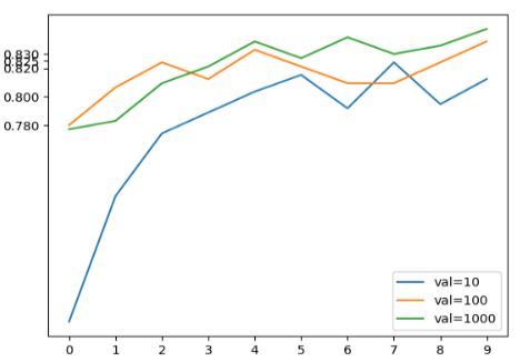
When we cannot see an improvement compared to the less complex model then it’s fine to go with this easier one. But in the next section we want to look at the effects of regularization and dropout so let’s use the more complex neural network for now.
