
This is the second part of Transfer Learning section. While in the last article we looked at reading image data this article covers the training part.
Transfer Learning – Part 2/2
Train Xception on smaller images (150×150) (Better to run it with a GPU)
So far for reading the data, now let’s train a model. base_model here means that we take the convolution part of the Xception model that was trained on ImageNet and then train our custom model on top of that. This will have 10 classes.
To only keep the convolutional layers there is a parameter include_top that we need to set to false. “top” could be a bit confusing, but Keras stacks layers conceptionally from bottom to top. That means on top there are the dense layers.
Next important point is we don’t want to train this model, we only want to use it for extracting the vector representation. With “base_model.trainable = False” we can define the model as not trainable. That means when we train our model, we don’t want to change the convolutional layers (=freezing the convolutional layers).
base_model = Xception(
    weights='imagenet',
    include_top=False,
    input_shape=(150, 150, 3)
)

base_model.trainable = False

# Output:
# Downloading data from https://storage.googleapis.com/tensorflow/keras-applications/xception/xception_weights_tf_dim_ordering_tf_kernels_notop.h5
83683744/83683744 [==============================] - 30s 0us/step
Next thing to do is creating a new top. First thing is specifying the input. Input is the part of the model that receive the images. This input then goes to the base model which we use to extract the vector representation.
inputs = keras.Input(shape=(150, 150, 3))
base = base_model(inputs)
outputs = base
model = keras.Model(inputs, outputs)
preds = model.predict(X)

# Output: 1/1 [==============================] - 3s 3s/step

preds.shape
# Output: (32, 5, 5, 2048)
What we get here is a 4-dimensional shape. 32 is the batch size. So for each image we’ve got a 5x5x2,048 representation which doesn’t look like a vector representation yet. So what we need to do now is turning this to a bunch of vectors. We can do this while chunking the 5x5x2048 representation in slices of size 5×5 and put the average of this 25 values to a one-dimensional vector. This reduction of dimensionality is called pooling. In this case here we use average pooling – more concrete we do a 2D average pooling. In Keras we can do this pooling as shown in the next snippet.
inputs = keras.Input(shape=(150, 150, 3))
base = base_model(inputs)

pooling = keras.layers.GlobalAveragePooling2D()
vectors = pooling(base)
outputs = vectors

model = keras.Model(inputs, outputs)
preds = model.predict(X)

# Output:
# WARNING:tensorflow:5 out of the last 6 calls to <function Model.make_predict_function.<locals>.predict_function at 0x7fa90c8fcf70> triggered tf.function retracing. Tracing is expensive and the excessive number of tracings could be due to (1) creating @tf.function repeatedly in a loop, (2) passing tensors with different shapes, (3) passing Python objects instead of tensors. For (1), please define your @tf.function outside of the loop. For (2), @tf.function has reduce_retracing=True option that can avoid unnecessary retracing. For (3), please refer to https://www.tensorflow.org/guide/function#controlling_retracing and https://www.tensorflow.org/api_docs/python/tf/function for  more details.
# 1/1 [==============================] - 3s 3s/step

preds.shape
# Output: (32, 2048)
# Shorter form in functional style. That's the way how we view the neural network.
inputs = keras.Input(shape=(150, 150, 3))

base = base_model(inputs)
vectors = keras.layers.GlobalAveragePooling2D()(base)
outputs = vectors
model = keras.Model(inputs, outputs)

preds = model.predict(X)
preds.shape

# Output:
# 1/1 [==============================] - 3s 3s/step
# (32, 2048)
We’re still not done yet. We have our vectors but now we need to put the dense layer on top of that to turn the vectors into predictions. What we want to have at the end is an array 32×10 with their predictions. That is what we call output. For turning vectors into outputs we want to create a dense layer.
| applying base model | pooling | |||||
| INPUTS | ==> | BASE | ==> | VECTORS | ==> | OUTPUTS |
| 32x150x150 | 32x5x5x2048 | 32×2048 | 32×10 |
inputs = keras.Input(shape=(150, 150, 3))

base = base_model(inputs)
vectors = keras.layers.GlobalAveragePooling2D()(base)
outputs = keras.layers.Dense(10)(vectors)
model = keras.Model(inputs, outputs)

preds = model.predict(X)
preds.shape

# Output:
# 1/1 [==============================] - 3s 3s/step
# (32, 10)
To summarize what we’ve done so far (for one image). We have our t-shirt (150x150x3) as input. Applying the base_model on inputs gives us the “base” (5x5x2048). Applying pooling on “base” we turn this into a one-dimensional vector (2048). On top of this we added the dense layer, which turns the vector representation into predictions. The dimensionality of this is 10 because we have 10 classes. This is what goes to the outputs variable. “outputs” is what we will have when we invoke predict and the input is the X.
base_model = Xception(
    weights='imagenet',
    include_top=False,
    input_shape=(150, 150, 3)
)

base_model.trainable = False
inputs = keras.Input(shape=(150, 150, 3))
base = base_model(inputs, training=False)
vectors = keras.layers.GlobalAveragePooling2D()(base)
outputs = keras.layers.Dense(10)(vectors)
model = keras.Model(inputs, outputs)

preds = model.predict(X)
preds.shape

# Output:
# 1/1 [==============================] - 2s 2s/step
# (32, 10)
preds[0]

# Output:
# array([-0.03203598,  1.0506403 ,  1.5579934 , -0.47385398, -0.23905472,
#              0.09166865, -1.2453439 , -0.7762855 ,  0.75367785,  0.5877316 ],
#              dtype=float32)
What’s important the model outputs here just random numbers because we haven’t trained the model yet. The reason for this is, when creating a dense layer it’s initialized with random numbers. That means we now have to train the model.
To train a model we need to have some things.
First we need an optimizer which finds the best weights for the model. For more information on optimizers look at the documentation. But also the CS231n course is a great reference for more information on that.
The learning rate here is similar to eta in case of XGBoost.
Then the optimizer needs to evaluate the changes are, therefor we need a concept that is called loss. Keras has some different kind of losses. Because we have a multi-class classification problem we use “CategoricalCrossentropy”. For binary classification problem we would use BinaryCrossentropy, and for regression problems we would use MeanSquaredError. CategoricalCrossentropy outputs just a number – the lower the better. The optimizer is trying to optimize this number to make it as low as possible. How the optimizer is doing this? The optimizer can change the parameters of the dense layers.
There is an important parameter “from_logits” which is set to “True”. The documentation says “Whether ‘y_pred’ is expected to be a logits tensor. By default, we assume that ‘y_pred’ encodes a probability distribution. Note: Using from_digits=True may be more numerically stable.”
Let’s try to explain what’s happening here.
When we talked about dense layers, then there was an input and an output layer. We applied softmax to this output. This softmax is called “activation”. It takes the output from the output layer as input and turns it into a probability. And exactly this input is called “logits” which is the raw output of the dense layer before applying softmax. If we have softmax then we have probabilities, if we don’t have softmax we have raw score. Here we want to use raw score so we set that value to True. That means we don’t use activation here. In case we need probabilities we can set that value to False. But then we must change the dense layer code from
outputs = keras.layers.Dense(10)(vectors) —> outputs = keras.layers.Dense(10, activation=’softmax’)(vectors)
But we stay with true and left the other code unchanged.
Now we need to compile the model before we can start training it. For compiling we need the optimizer and the loss that we defined before. We’re also interested in monitoring a special metric which is accuracy. At each step of training it will show the progress.
learning_rate = 0.01
optimizer = keras.optimizers.Adam(learning_rate=learning_rate)

loss = keras.losses.CategoricalCrossentropy(from_logits=True)

model.compile(optimizer=optimizer, loss=loss, metrics=['accuracy'])
Now everyrthing is ready for training the model. Here we use the model.fit method which need the training data, the epoch count for how many epochs the model should be trained and the validation data. One epoch means that we go over the whole training dataset once, not image by image, but in batches of size 32 as we have defined before. Last batch can be less than this predefined size of 32 images. When training a model we apply to one batch at a time and when it’s done for all batches we call this one epoch. 10 epoch for example means go over the data 10 times.
The output shows the current loss which is CategoricalCrossentropy and the accuracy for each epoch.
model.fit(train_ds, epochs=10, validation_data=val_ds)

# Output:
# Epoch 1/10
# 96/96 [==============================] - 152s 2s/step - loss: 1.3336 - accuracy: 0.6617 - val_loss: 0.7325 - val_accuracy: 0.7947
# Epoch 2/10
# 96/96 [==============================] - 163s 2s/step - loss: 0.5488 - accuracy: 0.8240 - val_loss: 0.8414 - val_accuracy: 0.7801
# Epoch 3/10
# 96/96 [==============================] - 125s 1s/step - loss: 0.3361 - accuracy: 0.8836 - val_loss: 0.7177 - val_accuracy: 0.7918
# Epoch 4/10
# 96/96 [==============================] - 121s 1s/step - loss: 0.2275 - accuracy: 0.9214 - val_loss: 0.7611 - val_accuracy: 0.8152
# Epoch 5/10
# 96/96 [==============================] - 148s 2s/step - loss: 0.1337 - accuracy: 0.9524 - val_loss: 0.7521 - val_accuracy: 0.8328
# Epoch 6/10
# 96/96 [==============================] - 147s 2s/step - loss: 0.1041 - accuracy: 0.9654 - val_loss: 0.8706 - val_accuracy: 0.8006
# Epoch 7/10
# 96/96 [==============================] - 141s 1s/step - loss: 0.0984 - accuracy: 0.9658 - val_loss: 0.9092 - val_accuracy: 0.7977
# Epoch 8/10
# 96/96 [==============================] - 151s 2s/step - loss: 0.0506 - accuracy: 0.9870 - val_loss: 0.7548 - val_accuracy: 0.8240
# Epoch 9/10
# 96/96 [==============================] - 137s 1s/step - loss: 0.0439 - accuracy: 0.9883 - val_loss: 0.8632 - val_accuracy: 0.8299
# Epoch 10/10
# 96/96 [==============================] - 137s 1s/step - loss: 0.0462 - accuracy: 0.9883 - val_loss: 0.8992 - val_accuracy: 0.8152
# <keras.src.callbacks.History at 0x7fa9012e9880>
This time we want to access the loss and accuracy values. In case of XGBoost we needed to capture the output but here we don’t need to do this because the model.fit method returns an history object which contains all this information.
history = model.fit(train_ds, epochs=10, validation_data=val_ds)

# Output:
# Epoch 1/10
# 96/96 [==============================] - 140s 1s/step - loss: 1.2547 - accuracy: 0.6799 - val_loss: 1.0608 - val_accuracy: 0.7185
# Epoch 2/10
# 96/96 [==============================] - 137s 1s/step - loss: 0.5159 - accuracy: 0.8295 - val_loss: 0.7736 - val_accuracy: 0.7947
# Epoch 3/10
# 96/96 [==============================] - 124s 1s/step - loss: 0.3355 - accuracy: 0.8797 - val_loss: 0.8798 - val_accuracy: 0.7859
# Epoch 4/10
# 96/96 [==============================] - 134s 1s/step - loss: 0.2076 - accuracy: 0.9263 - val_loss: 0.9194 - val_accuracy: 0.7771
# Epoch 5/10
# 96/96 [==============================] - 135s 1s/step - loss: 0.1612 - accuracy: 0.9423 - val_loss: 0.8815 - val_accuracy: 0.8182
# Epoch 6/10
# 96/96 [==============================] - 144s 1s/step - loss: 0.1053 - accuracy: 0.9606 - val_loss: 0.9155 - val_accuracy: 0.8123
# Epoch 7/10
# 96/96 [==============================] - 146s 2s/step - loss: 0.0855 - accuracy: 0.9743 - val_loss: 0.8817 - val_accuracy: 0.8123
# Epoch 8/10
# 96/96 [==============================] - 131s 1s/step - loss: 0.0440 - accuracy: 0.9915 - val_loss: 1.0533 - val_accuracy: 0.7977
# Epoch 9/10
# 96/96 [==============================] - 132s 1s/step - loss: 0.0590 - accuracy: 0.9788 - val_loss: 0.9280 - val_accuracy: 0.8094
# Epoch 10/10
# 96/96 [==============================] - 130s 1s/step - loss: 0.0474 - accuracy: 0.9853 - val_loss: 0.8992 - val_accuracy: 0.8152
The training loss is decreasing and the accuracy for validation in the first epoch is 72%. Comparing the training accuracy with the validation accuracy we see both values increasing over time until epoch 3. There is a discrepancy between both accuracy values. There is a difference of about 10%. Another thing is that training accuracy keeps improving but on the validation data not so much. That could mean that the model starts to overfit already. When we look at validation accuracy we see that it oscillates around 80%. In the same time the accuracy on training data is very high (it’s almost 1). That are really good signs for an overfitting model. The results are saved in the history object. We’re interested in training accuracy and validation accuracy.
history.history['accuracy']
#history.history['val_accuracy']

# Output:
# [0.6799217462539673,
#  0.829530656337738,
#  0.879726231098175,
#  0.9263363480567932,
#  0.942307710647583,
#  0.9605606198310852,
#  0.974250316619873,
#  0.991525411605835,
#  0.9788135886192322,
#  0.9853324890136719]
#plt.plot(history.history['accuracy'], label='train')
plt.plot(history.history['val_accuracy'], label='val')
plt.xticks(np.arange(10))
plt.legend()
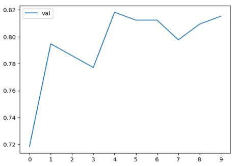
The first peak is after one epoch. Maybe the best model is after 4 epochs because the training accuracy is still not very high (<95%). But the model after one epoch is already quite ok. This value of almost 80% is a good one because it’s without any tuning. There are many parameters to tune. We’ll tune the most important one in the next section.
