
XGBoost parameter tuning – Part 2/2
This is the second part about XGBoost parameter tuning. In the first part, we tuned the first parameter – ‘eta‘. Now we will explore parameter tuning for ‘max_depth‘ and ‘min_child_weight‘. Finally, we’ll train the final model.
Tuning max_depth
max_depth=6
Now that we’ve set ‘eta‘ to 0.1, which we determined to be the best value, we’re going to focus on tuning the ‘max_depth‘ parameter. To do that, we’ll reset our scores dictionary to keep track of the new experiments. Initially, we’ll train a model with the same parameters as before, using it as a baseline for comparing different ‘max_depth‘ values.
scores = {}
%%capture output

xgb_params = {
    'eta': 0.1,
    'max_depth': 6,
    'min_child_weight': 1,

    'objective': 'binary:logistic',
    'eval_metric': 'auc',

    'nthread': 8,
    'seed': 1,
    'verbosity': 1,
}

model = xgb.train(xgb_params, dtrain, num_boost_round=200,
                  verbose_eval=5,
                  evals=watchlist)
key = 'max_depth=%s' % (xgb_params['max_depth'])
scores[key] = parse_xgb_output(output)
key

# Output: 'max_depth=6'
max_depth=3
Now, let’s set the ‘max_depth‘ value to 3.
%%capture output

xgb_params = {
    'eta': 0.1,
    'max_depth': 3,
    'min_child_weight': 1,

    'objective': 'binary:logistic',
    'eval_metric': 'auc',

    'nthread': 8,
    'seed': 1,
    'verbosity': 1,
}

model = xgb.train(xgb_params, dtrain, num_boost_round=200,
                  verbose_eval=5,
                  evals=watchlist)
key = 'max_depth=%s' % (xgb_params['max_depth'])
scores[key] = parse_xgb_output(output)
key

# Output: 'max_depth=3'
max_depth=4
Let’s go through the process once more for ‘max_depth=4‘.
%%capture output

xgb_params = {
    'eta': 0.1,
    'max_depth': 4,
    'min_child_weight': 1,

    'objective': 'binary:logistic',
    'eval_metric': 'auc',

    'nthread': 8,
    'seed': 1,
    'verbosity': 1,
}

model = xgb.train(xgb_params, dtrain, num_boost_round=200,
                  verbose_eval=5,
                  evals=watchlist)
key = 'max_depth=%s' % (xgb_params['max_depth'])
scores[key] = parse_xgb_output(output)
key

# Output: 'max_depth=4'
max_depth=10
Let’s repeat the process for ‘max_depth=10‘ once more.
%%capture output

xgb_params = {
    'eta': 0.1,
    'max_depth': 10,
    'min_child_weight': 1,

    'objective': 'binary:logistic',
    'eval_metric': 'auc',

    'nthread': 8,
    'seed': 1,
    'verbosity': 1,
}

model = xgb.train(xgb_params, dtrain, num_boost_round=200,
                  verbose_eval=5,
                  evals=watchlist)
key = 'max_depth=%s' % (xgb_params['max_depth'])
scores[key] = parse_xgb_output(output)
key

# Output: 'max_depth=10'
Plotting max_depth
Now that we’ve collected data from four runs, let’s plot this information and determine which model performs the best.
for max_depth, df_score in scores.items():
    plt.plot(df_score.num_iter, df_score.val_auc, label=max_depth)

#plt.ylim(0.8, 0.84)
plt.legend()

We see the depth of 10 is worst. So actually we can delete it by del scores['max_depth=10']
To get a better view on the y-area between 0.8 and 0.84 we can limit the plot as shown in the next snippet.
for max_depth, df_score in scores.items():
    plt.plot(df_score.num_iter, df_score.val_auc, label=max_depth)

plt.ylim(0.8, 0.84)
plt.legend()

‘max_depth = 6‘ is the second worst. We conclude that ‘max_depth‘ of 3 is the best depth for us.
Tuning min_child_weight
min_child_weight=1
Now, we’ll set ‘eta‘ to 0.1 and ‘max_depth‘ to 3. We’re ready to start tuning the last parameter, which is ‘min_child_weight.’ To do this, we need to reset our scores dictionary once again to track the new experiments. Initially, we’ll train a model with the same parameters as before, but we’ll set ‘min_child_weight‘ to 1. This model will serve as our baseline for comparing different ‘min_child_weight‘ values.
scores = {}
%%capture output

xgb_params = {
    'eta': 0.1,
    'max_depth': 3,
    'min_child_weight': 1,

    'objective': 'binary:logistic',
    'eval_metric': 'auc',

    'nthread': 8,
    'seed': 1,
    'verbosity': 1,
}

model = xgb.train(xgb_params, dtrain, num_boost_round=200,
                  verbose_eval=5,
                  evals=watchlist)
key = 'min_child_weight=%s' % (xgb_params['min_child_weight'])
scores[key] = parse_xgb_output(output)
key

# Output: 'min_child_weight=1'
min_child_weight=10
Now, let’s set the ‘min_child_weight‘ value to 10.
%%capture output

xgb_params = {
    'eta': 0.1,
    'max_depth': 3,
    'min_child_weight': 10,

    'objective': 'binary:logistic',
    'eval_metric': 'auc',

    'nthread': 8,
    'seed': 1,
    'verbosity': 1,
}

model = xgb.train(xgb_params, dtrain, num_boost_round=200,
                  verbose_eval=5,
                  evals=watchlist)
key = 'min_child_weight=%s' % (xgb_params['min_child_weight'])
scores[key] = parse_xgb_output(output)
key

# Output: 'min_child_weight=10'
min_child_weight=30
Let’s go through the process once more for ‘min_child_weight=30‘.
%%capture output

xgb_params = {
    'eta': 0.1,
    'max_depth': 3,
    'min_child_weight': 30,

    'objective': 'binary:logistic',
    'eval_metric': 'auc',

    'nthread': 8,
    'seed': 1,
    'verbosity': 1,
}

model = xgb.train(xgb_params, dtrain, num_boost_round=200,
                  verbose_eval=5,
                  evals=watchlist)
key = 'min_child_weight=%s' % (xgb_params['min_child_weight'])
scores[key] = parse_xgb_output(output)
key

# Output: 'min_child_weight=30'
Plotting min_child_weight
This should give us an idea if we actually need to increase this value or not. Now we can compare all runs of ‘min_child_weight=1‘, ‘min_child_weight=10‘, and ‘min_child_weight=30‘.
for min_child_weight, df_score in scores.items():
    plt.plot(df_score.num_iter, df_score.val_auc, label=min_child_weight)

plt.legend()

Here it’s not so easy to see which one is the best. We should also enlarge it a bit.
for min_child_weight, df_score in scores.items():
    plt.plot(df_score.num_iter, df_score.val_auc, label=min_child_weight)

plt.ylim(0.82, 0.84)
plt.legend()
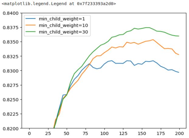
This plot shows some differences compared to the video by Alexey. In this plot, a ‘min_child_weight‘ of 30 appears to be the best-performing value, whereas in the video, the choice is ‘min_child_weight‘ of 1. To maintain consistency with the video’s results, I’ve opted to select a ‘min_child_weight‘ of 1. It’s worth noting that parameter tuning can be influenced by various factors, and flexibility in choosing the optimal values is important.
Train final model
To train the final model, we need to determine the number of iterations for training. In the video, Alexey chose to train for 175 iterations.
xgb_params = {
    'eta': 0.1,
    'max_depth': 3,
    'min_child_weight': 1,

    'objective': 'binary:logistic',
    'eval_metric': 'auc',

    'nthread': 8,
    'seed': 1,
    'verbosity': 1,
}

model = xgb.train(xgb_params, dtrain, num_boost_round=175)
xgb_params = {
    'eta': 0.1,
    'max_depth': 3,
    'min_child_weight': 30,

    'objective': 'binary:logistic',
    'eval_metric': 'auc',

    'nthread': 8,
    'seed': 1,
    'verbosity': 1,
}

model = xgb.train(xgb_params, dtrain, num_boost_round=175)
Always creating all these plots may not be necessary. You can also examine the raw output and use tools like pen and paper or an Excel spreadsheet when experimenting with parameter tuning. Finding the best approach depends on your preferences and needs. Eta, max_depth, and min_child_weight are indeed important parameters, but there are other valuable ones to consider.
For reference, you can explore the complete list of XGBoost parameters here: XGBoost Parameters.
Two parameters that can be particularly useful are ‘subsample‘ and ‘colsample_bytree.’ They have some similarities:
- ‘
colsample_bytree‘:
Similar to what we observe in Random Forest, this parameter controls how many features each tree gets to see at each iteration. The maximum value is 1.0. You can experiment with values like 0.3 and 0.6, and then fine-tune around those values. - ‘
subsample‘:
Instead of sampling columns, this parameter allows you to sample rows. It means you can choose to provide only a percentage of the training data. For example, setting it to 0.5 means you randomly select 50% of the training data.
In addition to these, there’s a wealth of information available on rules of thumb for tuning XGBoost parameters. Kaggle is a valuable resource for learning more, and you can find many tutorials on XGBoost parameter tuning.
