
XGBoost parameter tuning – Part 1/2
This part is about XGBoost parameter tuning. It’s the first part of a two-part series, where we begin by tuning the initial parameter – ‘eta‘. The subsequent article will explore parameter tuning for ‘max_depth‘ and ‘min_child_weight‘. In the final phase, we’ll train the final model. Let’s start tuning the first parameter.
Tuning Eta
Eta, also known as the learning rate, determines the influence of the following model when correcting the results of the previous model. If the weight is set to 1.0, all new predictions are used to correct the previous ones. However, when the weight is 0.3, only 30% of the new predictions are considered. In essence, eta governs the size of the steps taken during the learning process.
Now, let’s explore how different values of eta impact model performance. To facilitate this, we’ll create a dictionary called ‘scores‘ to store the performance scores for each value of eta.
Eta = 0.3
scores = {}
%%capture output

xgb_params = {
    'eta': 0.3,
    'max_depth': 6,
    'min_child_weight': 1,

    'objective': 'binary:logistic',
    'eval_metric': 'auc',

    'nthread': 8,
    'seed': 1,
    'verbosity': 1
}

model = xgb.train(xgb_params, dtrain, num_boost_round=200,
                 verbose_eval=5,
                 evals=watchlist)
We aim to structure keys in the format ‘eta=0.3’ to serve as identifiers in the scores dictionary.
'eta=%s' % (xgb_params['eta'])
# Output: 'eta=0.3'
In the next snippet, we once again employ the ‘parse_xgb_output‘ function, which we defined in the previous article. This function returns a dataframe that contains train_auc and val_auc values for different num_iter.
key = 'eta=%s' % (xgb_params['eta'])
scores[key] = parse_xgb_output(output)
key

# Output: 'eta=0.3'
Now the dictionary scores contains the dataframe for this eta.
scores

# Output:
# {'eta=0.3':     num_iter  train_auc  val_auc
#  0          0    0.86730  0.77938
#  1          5    0.93086  0.80858
#  2         10    0.95447  0.80851
#  3         15    0.96554  0.81334
#  4         20    0.97464  0.81729
#  5         25    0.97953  0.81686
#   ...
#  36       180    1.00000  0.80723
#  37       185    1.00000  0.80678
#  38       190    1.00000  0.80672
#  39       195    1.00000  0.80708
#  40       199    1.00000  0.80725}
scores['eta=0.3']
| num_iter | train_auc | val_auc | |
|---|---|---|---|
| 0 | 0 | 0.86730 | 0.77938 |
| 1 | 5 | 0.93086 | 0.80858 |
| 2 | 10 | 0.95447 | 0.80851 |
| 3 | 15 | 0.96554 | 0.81334 |
| 4 | 20 | 0.97464 | 0.81729 |
| 5 | 25 | 0.97953 | 0.81686 |
| 6 | 30 | 0.98579 | 0.81543 |
| 7 | 35 | 0.99011 | 0.81206 |
| 8 | 40 | 0.99421 | 0.80922 |
| 9 | 45 | 0.99548 | 0.80842 |
| 10 | 50 | 0.99653 | 0.80918 |
| 11 | 55 | 0.99765 | 0.81114 |
| 12 | 60 | 0.99817 | 0.81172 |
| 13 | 65 | 0.99887 | 0.80798 |
| 14 | 70 | 0.99934 | 0.80870 |
| 15 | 75 | 0.99965 | 0.80555 |
| 16 | 80 | 0.99979 | 0.80549 |
| 17 | 85 | 0.99988 | 0.80374 |
| 18 | 90 | 0.99993 | 0.80409 |
| 19 | 95 | 0.99996 | 0.80548 |
| 20 | 100 | 0.99998 | 0.80509 |
| 21 | 105 | 0.99999 | 0.80629 |
| 22 | 110 | 1.00000 | 0.80637 |
| 23 | 115 | 1.00000 | 0.80494 |
| 24 | 120 | 1.00000 | 0.80574 |
| 25 | 125 | 1.00000 | 0.80727 |
| 26 | 130 | 1.00000 | 0.80746 |
| 27 | 135 | 1.00000 | 0.80753 |
| 28 | 140 | 1.00000 | 0.80899 |
| 29 | 145 | 1.00000 | 0.80733 |
| 30 | 150 | 1.00000 | 0.80841 |
| 31 | 155 | 1.00000 | 0.80734 |
| 32 | 160 | 1.00000 | 0.80711 |
| 33 | 165 | 1.00000 | 0.80707 |
| 34 | 170 | 1.00000 | 0.80734 |
| 35 | 175 | 1.00000 | 0.80704 |
| 36 | 180 | 1.00000 | 0.80723 |
| 37 | 185 | 1.00000 | 0.80678 |
| 38 | 190 | 1.00000 | 0.80672 |
| 39 | 195 | 1.00000 | 0.80708 |
| 40 | 199 | 1.00000 | 0.80725 |
Eta = 1.0
Now, let’s set the eta value to its maximum, which is 1.0.
%%capture output

xgb_params = {
    'eta': 1.0,
    'max_depth': 6,
    'min_child_weight': 1,

    'objective': 'binary:logistic',
    'eval_metric': 'auc',

    'nthread': 8,
    'seed': 1,
    'verbosity': 1,
}

model = xgb.train(xgb_params, dtrain, num_boost_round=200,
                  verbose_eval=5,
                  evals=watchlist)
key = 'eta=%s' % (xgb_params['eta'])
scores[key] = parse_xgb_output(output)
key
# Output: 'eta=1.0'
With the updated eta value, the scores dictionary should now encompass two values and two corresponding keys.
scores['eta=1.0']
| num_iter | train_auc | val_auc | |
|---|---|---|---|
| 0 | 0 | 0.86730 | 0.77938 |
| 1 | 5 | 0.95857 | 0.79136 |
| 2 | 10 | 0.98061 | 0.78355 |
| 3 | 15 | 0.99549 | 0.78050 |
| 4 | 20 | 0.99894 | 0.78591 |
| 5 | 25 | 0.99989 | 0.78401 |
| 6 | 30 | 1.00000 | 0.78371 |
| 7 | 35 | 1.00000 | 0.78234 |
| 8 | 40 | 1.00000 | 0.78184 |
| 9 | 45 | 1.00000 | 0.77963 |
| 10 | 50 | 1.00000 | 0.78645 |
| 11 | 55 | 1.00000 | 0.78644 |
| 12 | 60 | 1.00000 | 0.78545 |
| 13 | 65 | 1.00000 | 0.78612 |
| 14 | 70 | 1.00000 | 0.78515 |
| 15 | 75 | 1.00000 | 0.78516 |
| 16 | 80 | 1.00000 | 0.78420 |
| 17 | 85 | 1.00000 | 0.78570 |
| 18 | 90 | 1.00000 | 0.78793 |
| 19 | 95 | 1.00000 | 0.78865 |
| 20 | 100 | 1.00000 | 0.79075 |
| 21 | 105 | 1.00000 | 0.79107 |
| 22 | 110 | 1.00000 | 0.79022 |
| 23 | 115 | 1.00000 | 0.79036 |
| 24 | 120 | 1.00000 | 0.79021 |
| 25 | 125 | 1.00000 | 0.79025 |
| 26 | 130 | 1.00000 | 0.78994 |
| 27 | 135 | 1.00000 | 0.79084 |
| 28 | 140 | 1.00000 | 0.79048 |
| 29 | 145 | 1.00000 | 0.78967 |
| 30 | 150 | 1.00000 | 0.78969 |
| 31 | 155 | 1.00000 | 0.78992 |
| 32 | 160 | 1.00000 | 0.79064 |
| 33 | 165 | 1.00000 | 0.79067 |
| 34 | 170 | 1.00000 | 0.79115 |
| 35 | 175 | 1.00000 | 0.79126 |
| 36 | 180 | 1.00000 | 0.79199 |
| 37 | 185 | 1.00000 | 0.79179 |
| 38 | 190 | 1.00000 | 0.79165 |
| 39 | 195 | 1.00000 | 0.79201 |
| 40 | 199 | 1.00000 | 0.79199 |
Eta = 0.1
Let’s go through the process once more for ‘eta=0.1’ and subsequently print out the dataframe.
%%capture output

xgb_params = {
    'eta': 0.1,
    'max_depth': 6,
    'min_child_weight': 1,

    'objective': 'binary:logistic',
    'eval_metric': 'auc',

    'nthread': 8,
    'seed': 1,
    'verbosity': 1,
}

model = xgb.train(xgb_params, dtrain, num_boost_round=200,
                  verbose_eval=5,
                  evals=watchlist)
key = 'eta=%s' % (xgb_params['eta'])
scores[key] = parse_xgb_output(output)
key

# Output: 'eta=0.1'
scores['eta=0.1']
| num_iter | train_auc | val_auc | |
|---|---|---|---|
| 0 | 0 | 0.86730 | 0.77938 |
| 1 | 5 | 0.90325 | 0.79290 |
| 2 | 10 | 0.91874 | 0.80510 |
| 3 | 15 | 0.93126 | 0.81380 |
| 4 | 20 | 0.93873 | 0.81804 |
| 5 | 25 | 0.94638 | 0.82065 |
| 6 | 30 | 0.95338 | 0.82063 |
| 7 | 35 | 0.95874 | 0.82404 |
| 8 | 40 | 0.96325 | 0.82644 |
| 9 | 45 | 0.96694 | 0.82602 |
| 10 | 50 | 0.97195 | 0.82549 |
| 11 | 55 | 0.97475 | 0.82648 |
| 12 | 60 | 0.97708 | 0.82781 |
| 13 | 65 | 0.97937 | 0.82775 |
| 14 | 70 | 0.98214 | 0.82681 |
| 15 | 75 | 0.98315 | 0.82728 |
| 16 | 80 | 0.98517 | 0.82560 |
| 17 | 85 | 0.98721 | 0.82503 |
| 18 | 90 | 0.98840 | 0.82443 |
| 19 | 95 | 0.98972 | 0.82389 |
| 20 | 100 | 0.99061 | 0.82456 |
| 21 | 105 | 0.99157 | 0.82359 |
| 22 | 110 | 0.99224 | 0.82274 |
| 23 | 115 | 0.99288 | 0.82147 |
| 24 | 120 | 0.99378 | 0.82154 |
| 25 | 125 | 0.99481 | 0.82195 |
| 26 | 130 | 0.99541 | 0.82252 |
| 27 | 135 | 0.99564 | 0.82190 |
| 28 | 140 | 0.99630 | 0.82219 |
| 29 | 145 | 0.99673 | 0.82177 |
| 30 | 150 | 0.99711 | 0.82136 |
| 31 | 155 | 0.99750 | 0.82154 |
| 32 | 160 | 0.99774 | 0.82102 |
| 33 | 165 | 0.99821 | 0.82060 |
| 34 | 170 | 0.99838 | 0.82060 |
| 35 | 175 | 0.99861 | 0.82012 |
| 36 | 180 | 0.99882 | 0.82053 |
| 37 | 185 | 0.99898 | 0.82028 |
| 38 | 190 | 0.99904 | 0.81973 |
| 39 | 195 | 0.99920 | 0.81909 |
| 40 | 199 | 0.99927 | 0.81864 |
Eta = 0.05
Let’s do it again for ‘eta=0.05’ and print out the dataframe.
%%capture output

xgb_params = {
    'eta': 0.05,
    'max_depth': 6,
    'min_child_weight': 1,

    'objective': 'binary:logistic',
    'eval_metric': 'auc',

    'nthread': 8,
    'seed': 1,
    'verbosity': 1,
}

model = xgb.train(xgb_params, dtrain, num_boost_round=200,
                  verbose_eval=5,
                  evals=watchlist)
key = 'eta=%s' % (xgb_params['eta'])
scores[key] = parse_xgb_output(output)
key

# Output: 'eta=0.05'
scores['eta=0.05']
| num_iter | train_auc | val_auc | |
|---|---|---|---|
| 0 | 0 | 0.86730 | 0.77938 |
| 1 | 5 | 0.88650 | 0.79584 |
| 2 | 10 | 0.90368 | 0.79623 |
| 3 | 15 | 0.91072 | 0.79938 |
| 4 | 20 | 0.91774 | 0.80510 |
| 5 | 25 | 0.92385 | 0.80895 |
| 6 | 30 | 0.92987 | 0.81175 |
| 7 | 35 | 0.93379 | 0.81480 |
| 8 | 40 | 0.93856 | 0.81547 |
| 9 | 45 | 0.94316 | 0.81807 |
| 10 | 50 | 0.94753 | 0.81793 |
| 11 | 55 | 0.95028 | 0.81926 |
| 12 | 60 | 0.95324 | 0.81998 |
| 13 | 65 | 0.95581 | 0.82159 |
| 14 | 70 | 0.95762 | 0.82299 |
| 15 | 75 | 0.95944 | 0.82368 |
| 16 | 80 | 0.96100 | 0.82524 |
| 17 | 85 | 0.96308 | 0.82604 |
| 18 | 90 | 0.96572 | 0.82666 |
| 19 | 95 | 0.96798 | 0.82667 |
| 20 | 100 | 0.96955 | 0.82719 |
| 21 | 105 | 0.97133 | 0.82745 |
| 22 | 110 | 0.97288 | 0.82819 |
| 23 | 115 | 0.97426 | 0.82822 |
| 24 | 120 | 0.97578 | 0.82768 |
| 25 | 125 | 0.97702 | 0.82790 |
| 26 | 130 | 0.97788 | 0.82760 |
| 27 | 135 | 0.97923 | 0.82764 |
| 28 | 140 | 0.98012 | 0.82725 |
| 29 | 145 | 0.98113 | 0.82665 |
| 30 | 150 | 0.98190 | 0.82575 |
| 31 | 155 | 0.98285 | 0.82581 |
| 32 | 160 | 0.98381 | 0.82560 |
| 33 | 165 | 0.98457 | 0.82576 |
| 34 | 170 | 0.98541 | 0.82591 |
| 35 | 175 | 0.98652 | 0.82581 |
| 36 | 180 | 0.98711 | 0.82526 |
| 37 | 185 | 0.98789 | 0.82525 |
| 38 | 190 | 0.98876 | 0.82535 |
| 39 | 195 | 0.98932 | 0.82538 |
| 40 | 199 | 0.98977 | 0.82522 |
Eta = 0.01
Once more, let’s assess the performance for ‘eta=0.01’.
%%capture output

xgb_params = {
    'eta': 0.01,
    'max_depth': 6,
    'min_child_weight': 1,

    'objective': 'binary:logistic',
    'eval_metric': 'auc',

    'nthread': 8,
    'seed': 1,
    'verbosity': 1,
}

model = xgb.train(xgb_params, dtrain, num_boost_round=200,
                  verbose_eval=5,
                  evals=watchlist)
key = 'eta=%s' % (xgb_params['eta'])
scores[key] = parse_xgb_output(output)
key

# Output: 'eta=0.01'
scores['eta=0.01']
| num_iter | train_auc | val_auc | |
|---|---|---|---|
| 0 | 0 | 0.86730 | 0.77938 |
| 1 | 5 | 0.87157 | 0.77925 |
| 2 | 10 | 0.87247 | 0.78051 |
| 3 | 15 | 0.87541 | 0.78302 |
| 4 | 20 | 0.87584 | 0.78707 |
| 5 | 25 | 0.88406 | 0.79331 |
| 6 | 30 | 0.89027 | 0.79763 |
| 7 | 35 | 0.89559 | 0.79914 |
| 8 | 40 | 0.89782 | 0.79883 |
| 9 | 45 | 0.89983 | 0.79845 |
| 10 | 50 | 0.90182 | 0.79697 |
| 11 | 55 | 0.90394 | 0.79775 |
| 12 | 60 | 0.90531 | 0.79684 |
| 13 | 65 | 0.90630 | 0.79616 |
| 14 | 70 | 0.90796 | 0.79672 |
| 15 | 75 | 0.90955 | 0.79807 |
| 16 | 80 | 0.91116 | 0.79976 |
| 17 | 85 | 0.91227 | 0.80130 |
| 18 | 90 | 0.91368 | 0.80285 |
| 19 | 95 | 0.91515 | 0.80390 |
| 20 | 100 | 0.91654 | 0.80499 |
| 21 | 105 | 0.91791 | 0.80534 |
| 22 | 110 | 0.91902 | 0.80523 |
| 23 | 115 | 0.92032 | 0.80515 |
| 24 | 120 | 0.92135 | 0.80497 |
| 25 | 125 | 0.92262 | 0.80520 |
| 26 | 130 | 0.92405 | 0.80605 |
| 27 | 135 | 0.92547 | 0.80692 |
| 28 | 140 | 0.92667 | 0.80730 |
| 29 | 145 | 0.92771 | 0.80818 |
| 30 | 150 | 0.92919 | 0.80928 |
| 31 | 155 | 0.92990 | 0.81039 |
| 32 | 160 | 0.93077 | 0.81125 |
| 33 | 165 | 0.93155 | 0.81160 |
| 34 | 170 | 0.93246 | 0.81189 |
| 35 | 175 | 0.93348 | 0.81257 |
| 36 | 180 | 0.93466 | 0.81340 |
| 37 | 185 | 0.93585 | 0.81429 |
| 38 | 190 | 0.93685 | 0.81481 |
| 39 | 195 | 0.93777 | 0.81554 |
| 40 | 199 | 0.93862 | 0.81575 |
Plotting Eta
Now that we’ve inserted key-value pairs and gathered information from different runs, we can examine the keys in the dictionary. Next we can compare all runs of ‘eta=0.3’, ‘eta=1.0’, ‘eta=0.1’, ‘eta=0.05’, and ‘eta=0.01’.
scores.keys()
# Output: dict_keys(['eta=0.3', 'eta=1.0', 'eta=0.1', 'eta=0.05', 'eta=0.01'])
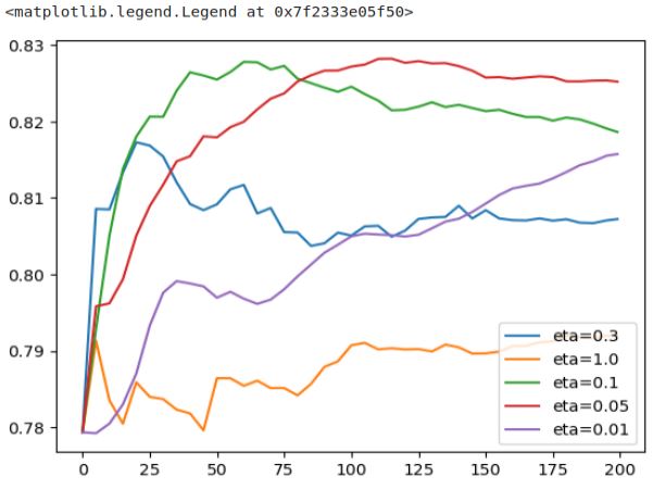
Let’s plot the information of our runs.
for key, df_score in scores.items():
    plt.plot(df_score.num_iter, df_score.val_auc, label=key)
plt.legend()
Let’s concentrate on a few graphs for the initial analysis. We will plot three of them: ‘eta=1.0’, ‘eta=0.3’, and ‘eta=0.1’.
etas = ['eta=1.0', 'eta=0.3', 'eta=0.1']
for eta in etas:
    df_score = scores[eta]
    plt.plot(df_score.num_iter, df_score.val_auc, label=eta)
plt.legend()
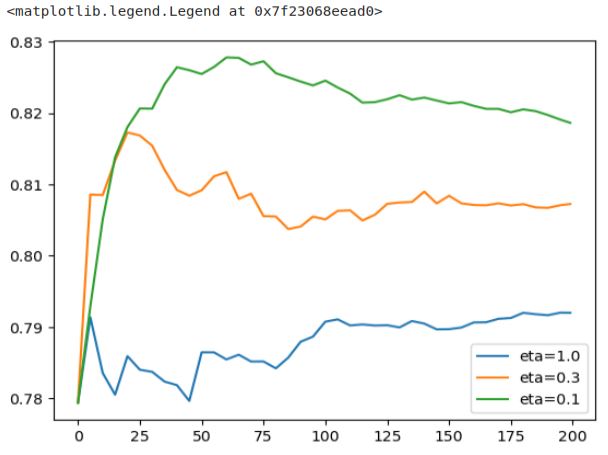
This plot provides a clearer view of the results. Notably, ‘eta=1.0’ exhibits the worst performance. It quickly reaches peak performance but then experiences a sharp decline, maintaining a consistently poor level. ‘eta=0.3’ performs reasonably well until around iteration 25, after which it steadily deteriorates. On the other hand, ‘eta=0.1’ demonstrates a slower growth rate, reaching its peak at a later stage before descending. This pattern is a direct reflection of the learning rate’s influence.
The learning rate controls both the speed at which the model learns and the size of the steps it takes during each iteration. If the steps are too large, the model learns rapidly but eventually starts to degrade due to the excessive step size, resulting in overfitting. Conversely, a smaller learning rate signifies slower but more stable learning. Such models tend to degrade more gradually, and their overfitting tendencies are less pronounced compared to models with higher learning rates.
Next let’s look at eta=0.3, eta=0.1, and eta=0.01
etas = ['eta=0.3', 'eta=0.1', 'eta=0.01']
for eta in etas:
    df_score = scores[eta]
    plt.plot(df_score.num_iter, df_score.val_auc, label=eta)
plt.legend()
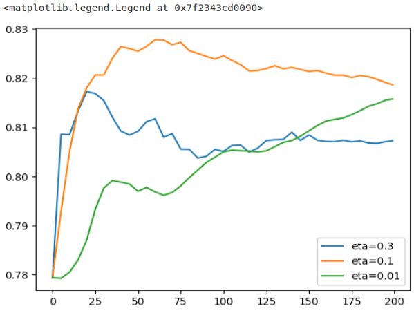
‘eta=0.01’ displays an extremely slow learning rate, making it challenging to estimate how long it might take to outperform the other model (represented by the orange curve). This model’s progress is painstakingly slow, as the steps it takes are exceedingly tiny.
On the other hand, ‘eta=0.3’ takes a few significant steps initially but succumbs to overfitting more rapidly. In this plot, ‘eta=0.1’ seems to strike the ideal balance, particularly between 50 and 75 iterations. It may take a bit longer to reach its peak performance, but the resulting performance improvement justifies the wait.
There was also eta=0.05 let’s finally look also at this plot.
etas = ['eta=0.1', 'eta=0.05', 'eta=0.01']
for eta in etas:
    df_score = scores[eta]
    plt.plot(df_score.num_iter, df_score.val_auc, label=eta)
plt.legend()
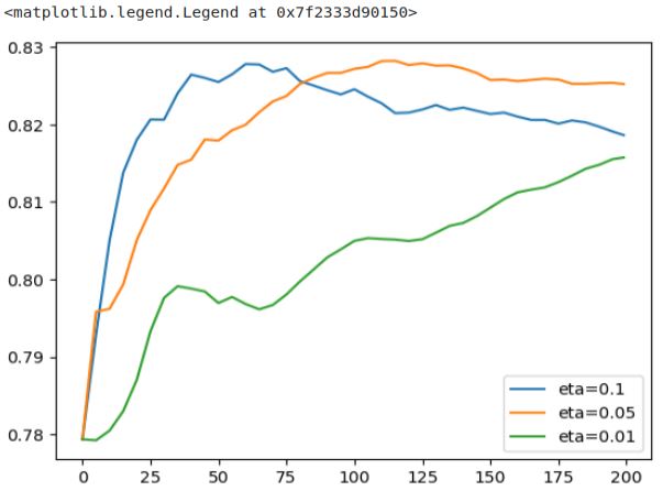
The ‘eta=0.05’ model requires approximately twice as many iterations to converge when compared to the blue model (‘eta=0.1’). Although it takes smaller steps and requires more time, the end result is still inferior to the blue model. Thus, it’s evident that the ‘eta=0.1’ model stands out as the best option, as it achieves better performance with fewer steps.
Now that we’ve found the best value for ‘eta,’ in the second part of XGBoost parameter tuning, we’ll focus on tuning two more parameters: ‘max_depth‘ and ‘min_child_weight‘ before proceeding to train the final model.
