Gradient boosting and XGBoost – Part 2/2
This is part 2 of ‘Gradient boosting and XGBoost.’ In the first part, we compared random forests and gradient boosting, followed by the installation of XGBoost and training our first XGBoost model. In this chapter, we delve into performance monitoring.
Performance Monitoring
In XGBoost, it’s feasible to monitor the performance of the training process, allowing us to closely observe each stage of the training procedure. To achieve this, after each iteration where a new tree is trained, we can promptly evaluate its performance on our validation data to assess the results. For this purpose, we can establish a watchlist that comprises the datasets we intend to use for evaluation.
watchlist = [(dtrain, 'train'), (dval, 'val')]
By default, XGBoost displays the error rate (logloss), a metric commonly used for parameter tuning. However, given the technical nature of this metric, we’ll opt for another more accessible metric for our analysis.
xgb_params = {
    'eta': 0.3,
    'max_depth': 6,
    'min_child_weight': 1,

    'objective': 'binary:logistic',

    'nthread': 8,
    'seed': 1,
    'verbosity': 1,
}

model = xgb.train(xgb_params, dtrain, num_boost_round=200,
                  evals=watchlist)

# Output:
# [0]	train-logloss:0.49703	val-logloss:0.54305
# [1]	train-logloss:0.44463	val-logloss:0.51462
# [2]	train-logloss:0.40707	val-logloss:0.49896
# [3]	train-logloss:0.37760	val-logloss:0.48654
# [4]	train-logloss:0.35990	val-logloss:0.48007
# [5]	train-logloss:0.33931	val-logloss:0.47563
# [6]	train-logloss:0.32586	val-logloss:0.47413
# [7]	train-logloss:0.31409	val-logloss:0.47702
# [8]	train-logloss:0.29962	val-logloss:0.48205
# [9]	train-logloss:0.29216	val-logloss:0.47996
# [10]	train-logloss:0.28407	val-logloss:0.47969
# ...
# [195]	train-logloss:0.02736	val-logloss:0.67492
# [196]	train-logloss:0.02728	val-logloss:0.67518
# [197]	train-logloss:0.02693	val-logloss:0.67791
# [198]	train-logloss:0.02665	val-logloss:0.67965
# [199]	train-logloss:0.02642	val-logloss:0.68022
For our monitoring purposes, we choose to use AUC as the metric, which we’ve previously employed. To do this, we set the eval_metric parameter to auc.
xgb_params = {
    'eta': 0.3,
    'max_depth': 6,
    'min_child_weight': 1,

    'objective': 'binary:logistic',
    'eval_metric': 'auc',

    'nthread': 8,
    'seed': 1,
    'verbosity': 1,
}

model = xgb.train(xgb_params, dtrain, num_boost_round=200,
                  evals=watchlist)

# Output:
# [0]	train-auc:0.86730	val-auc:0.77938
# [1]	train-auc:0.89140	val-auc:0.78964
# [2]	train-auc:0.90699	val-auc:0.79010
# [3]	train-auc:0.91677	val-auc:0.79967
# [4]	train-auc:0.92246	val-auc:0.80443
# [5]	train-auc:0.93086	val-auc:0.80858
# [6]	train-auc:0.93675	val-auc:0.80981
# [7]	train-auc:0.94108	val-auc:0.80872
# [8]	train-auc:0.94809	val-auc:0.80456
# [9]	train-auc:0.95100	val-auc:0.80653
# [10]	train-auc:0.95447	val-auc:0.80851
# ...
# [195]	train-auc:1.00000	val-auc:0.80708
# [196]	train-auc:1.00000	val-auc:0.80759
# [197]	train-auc:1.00000	val-auc:0.80718
# [198]	train-auc:1.00000	val-auc:0.80719
# [199]	train-auc:1.00000	val-auc:0.80725
The AUC on the training data reaches perfect accuracy (equal to one), but on the validation data, the performance remains relatively stable at around 80%. This suggests that the model may be overfitting.
To make this output more user-friendly, it would be beneficial to visualize it. Instead of printing output for every epoch, we can use verbose_eval=5 to display results only for every 5th epoch, making the monitoring process more manageable.
xgb_params = {
    'eta': 0.3,
    'max_depth': 6,
    'min_child_weight': 1,

    'objective': 'binary:logistic',
    'eval_metric': 'auc',

    'nthread': 8,
    'seed': 1,
    'verbosity': 1,
}

model = xgb.train(xgb_params, dtrain, num_boost_round=200,
                  verbose_eval=5,
                  evals=watchlist)

# Output:
# [0]	    train-auc:0.86730	val-auc:0.77938
# [5]	    train-auc:0.93086	val-auc:0.80858
# [10]	    train-auc:0.95447	val-auc:0.80851
# [15]	    train-auc:0.96554	val-auc:0.81334
# [20]	    train-auc:0.97464	val-auc:0.81729
# [25]	    train-auc:0.97953	val-auc:0.81686
# [30]	    train-auc:0.98579	val-auc:0.81543
# [35]	    train-auc:0.99011	val-auc:0.81206
# [40]	    train-auc:0.99421	val-auc:0.80922
# [45]	    train-auc:0.99548	val-auc:0.80842
# [50]	    train-auc:0.99653	val-auc:0.80918
# [55]	    train-auc:0.99765	val-auc:0.81114
# [60]	    train-auc:0.99817	val-auc:0.81172
# [65]	    train-auc:0.99887	val-auc:0.80798
# [70]	    train-auc:0.99934	val-auc:0.80870
# [75]	    train-auc:0.99965	val-auc:0.80555
# [80]	    train-auc:0.99979	val-auc:0.80549
# [85]	    train-auc:0.99988	val-auc:0.80374
# [90]	    train-auc:0.99993	val-auc:0.80409
# [95]	    train-auc:0.99996	val-auc:0.80548
# [100]	train-auc:0.99998	val-auc:0.80509
# [105]	train-auc:0.99999	val-auc:0.80629
# [110]	    train-auc:1.00000	val-auc:0.80637
# [115]	    train-auc:1.00000	val-auc:0.80494
# [120]	train-auc:1.00000	val-auc:0.80574
# [125]	train-auc:1.00000	val-auc:0.80727
# [130]	train-auc:1.00000	val-auc:0.80746
# [135]	train-auc:1.00000	val-auc:0.80753
# [140]	train-auc:1.00000	val-auc:0.80899
# [145]	train-auc:1.00000	val-auc:0.80733
# [150]	train-auc:1.00000	val-auc:0.80841
# [155]	train-auc:1.00000	val-auc:0.80734
# [160]	train-auc:1.00000	val-auc:0.80711
# [165]	train-auc:1.00000	val-auc:0.80707
# [170]	train-auc:1.00000	val-auc:0.80734
# [175]	train-auc:1.00000	val-auc:0.80704
# [180]	train-auc:1.00000	val-auc:0.80723
# [185]	train-auc:1.00000	val-auc:0.80678
# [190]	train-auc:1.00000	val-auc:0.80672
# [195]	train-auc:1.00000	val-auc:0.80708
# [199]	train-auc:1.00000	val-auc:0.80725
Parsing xgboost’s monitoring output
When you’re interested in visualizing this information on a plot, one of the challenges with XGBoost is that it doesn’t provide an easy way to extract this information since it’s printed to standard output. However, in Jupyter Notebook, there’s a method to capture whatever is printed to standard output and manipulate it. You can use the command %%capture output to achieve this. It captures all the content that the code outputs into a special object, which you can then use to extract the information. It’s worth noting that although something is happening in the code, we won’t see any output because it’s being captured.
%%capture output

xgb_params = {
    'eta': 0.3,
    'max_depth': 6,
    'min_child_weight': 1,

    'objective': 'binary:logistic',
    'eval_metric': 'auc',

    'nthread': 8,
    'seed': 1,
    'verbosity': 1,
}

model = xgb.train(xgb_params, dtrain, num_boost_round=200,
                  verbose_eval=5,
                  evals=watchlist)
s = output.stdout

print(s)
# Output:
# [0]	    train-auc:0.86730	val-auc:0.77938
# [5]	    train-auc:0.93086	val-auc:0.80858
# [10]	    train-auc:0.95447	val-auc:0.80851
# [15]	    train-auc:0.96554	val-auc:0.81334
# [20]	    train-auc:0.97464	val-auc:0.81729
# [25]	    train-auc:0.97953	val-auc:0.81686
# [30]	    train-auc:0.98579	val-auc:0.81543
# [35]	    train-auc:0.99011	val-auc:0.81206
# [40]	    train-auc:0.99421	val-auc:0.80922
# [45]	    train-auc:0.99548	val-auc:0.80842
# [50]	    train-auc:0.99653	val-auc:0.80918
# [55]	    train-auc:0.99765	val-auc:0.81114
# [60]	    train-auc:0.99817	val-auc:0.81172
# [65]	    train-auc:0.99887	val-auc:0.80798
# [70]	    train-auc:0.99934	val-auc:0.80870
# [75]	    train-auc:0.99965	val-auc:0.80555
# [80]	    train-auc:0.99979	val-auc:0.80549
# [85]	    train-auc:0.99988	val-auc:0.80374
# [90]	    train-auc:0.99993	val-auc:0.80409
# [95]	    train-auc:0.99996	val-auc:0.80548
# [100]	train-auc:0.99998	val-auc:0.80509
# [105]	train-auc:0.99999	val-auc:0.80629
# [110]	    train-auc:1.00000	val-auc:0.80637
# [115]	    train-auc:1.00000	val-auc:0.80494
# [120]	train-auc:1.00000	val-auc:0.80574
# [125]	train-auc:1.00000	val-auc:0.80727
# [130]	train-auc:1.00000	val-auc:0.80746
# [135]	train-auc:1.00000	val-auc:0.80753
# [140]	train-auc:1.00000	val-auc:0.80899
# [145]	train-auc:1.00000	val-auc:0.80733
# [150]	train-auc:1.00000	val-auc:0.80841
# [155]	train-auc:1.00000	val-auc:0.80734
# [160]	train-auc:1.00000	val-auc:0.80711
# [165]	train-auc:1.00000	val-auc:0.80707
# [170]	train-auc:1.00000	val-auc:0.80734
# [175]	train-auc:1.00000	val-auc:0.80704
# [180]	train-auc:1.00000	val-auc:0.80723
# [185]	train-auc:1.00000	val-auc:0.80678
# [190]	train-auc:1.00000	val-auc:0.80672
# [195]	train-auc:1.00000	val-auc:0.80708
# [199]	train-auc:1.00000	val-auc:0.80725
Now that we have the captured output in a string, the first step is to split it into individual lines by using the new line operator \n. The result is a string for each line of the output.
s.split('\n')

# Output:
# ['[0]\ttrain-auc:0.86730\tval-auc:0.77938',
#  '[5]\ttrain-auc:0.93086\tval-auc:0.80858',
#  '[10]\ttrain-auc:0.95447\tval-auc:0.80851',
#  '[15]\ttrain-auc:0.96554\tval-auc:0.81334',
#  '[20]\ttrain-auc:0.97464\tval-auc:0.81729',
#  '[25]\ttrain-auc:0.97953\tval-auc:0.81686',
#  '[30]\ttrain-auc:0.98579\tval-auc:0.81543',
#  '[35]\ttrain-auc:0.99011\tval-auc:0.81206',
#  '[40]\ttrain-auc:0.99421\tval-auc:0.80922',
#  '[45]\ttrain-auc:0.99548\tval-auc:0.80842',
#  '[50]\ttrain-auc:0.99653\tval-auc:0.80918',
#  '[55]\ttrain-auc:0.99765\tval-auc:0.81114',
#  '[60]\ttrain-auc:0.99817\tval-auc:0.81172',
#  '[65]\ttrain-auc:0.99887\tval-auc:0.80798',
#  '[70]\ttrain-auc:0.99934\tval-auc:0.80870',
#  '[75]\ttrain-auc:0.99965\tval-auc:0.80555',
#  '[80]\ttrain-auc:0.99979\tval-auc:0.80549',
#  '[85]\ttrain-auc:0.99988\tval-auc:0.80374',
#  '[90]\ttrain-auc:0.99993\tval-auc:0.80409',
#  '[95]\ttrain-auc:0.99996\tval-auc:0.80548',
#  '[100]\ttrain-auc:0.99998\tval-auc:0.80509',
#  '[105]\ttrain-auc:0.99999\tval-auc:0.80629',
#  '[110]\ttrain-auc:1.00000\tval-auc:0.80637',
#  '[115]\ttrain-auc:1.00000\tval-auc:0.80494',
#  '[120]\ttrain-auc:1.00000\tval-auc:0.80574',
#  '[125]\ttrain-auc:1.00000\tval-auc:0.80727',
#  '[130]\ttrain-auc:1.00000\tval-auc:0.80746',
#  '[135]\ttrain-auc:1.00000\tval-auc:0.80753',
#  '[140]\ttrain-auc:1.00000\tval-auc:0.80899',
#  '[145]\ttrain-auc:1.00000\tval-auc:0.80733',
#  '[150]\ttrain-auc:1.00000\tval-auc:0.80841',
#  '[155]\ttrain-auc:1.00000\tval-auc:0.80734',
#  '[160]\ttrain-auc:1.00000\tval-auc:0.80711',
#  '[165]\ttrain-auc:1.00000\tval-auc:0.80707',
#  '[170]\ttrain-auc:1.00000\tval-auc:0.80734',
#  '[175]\ttrain-auc:1.00000\tval-auc:0.80704',
#  '[180]\ttrain-auc:1.00000\tval-auc:0.80723',
#  '[185]\ttrain-auc:1.00000\tval-auc:0.80678',
#  '[190]\ttrain-auc:1.00000\tval-auc:0.80672',
#  '[195]\ttrain-auc:1.00000\tval-auc:0.80708',
#  '[199]\ttrain-auc:1.00000\tval-auc:0.80725',
# '']
Each line consists of three components: the number of iterations, the evaluation on the training dataset, and the evaluation on the validation dataset. We can split these components using the tabulator operator \t, resulting in three separate components. To ensure the correct format (integer, float, float), we utilize the strip method and perform the necessary string-to-integer and string-to-float conversions. The following snippet demonstrates these steps.
line = s.split('\n')[0]
line
# Output: '[0]\ttrain-auc:0.86730\tval-auc:0.77938'

line.split('\t')
# Output: ['[0]', 'train-auc:0.86730', 'val-auc:0.77938']

num_iter, train_auc, val_auc = line.split('\t')
num_iter, train_auc, val_auc
# Output: ('[0]', 'train-auc:0.86730', 'val-auc:0.77938')

int(num_iter.strip('[]'))
# Output: 0
float(train_auc.split(':')[1])
# Output: 0.8673
float(val_auc.split(':')[1])
# Output: 0.77938
We can combine all these steps to transform the information (number of iterations, AUC on the training data, and AUC on the validation data) from the output into a dataframe. The following snippet encapsulates all these steps within a single function for ease of use. This allows us to plot the data and perform further analysis.
def parse_xgb_output(output):
    results = []

    for line in output.stdout.strip().split('\n'):
        it_line, train_line, val_line = line.split('\t')

        it = int(it_line.strip('[]'))
        train = float(train_line.split(':')[1])
        val = float(val_line.split(':')[1])

        results.append((it, train, val))

    columns = ['num_iter', 'train_auc', 'val_auc']
    df_results = pd.DataFrame(results, columns=columns)
    return df_results
Now, let’s see how the function works in action.
df_score = parse_xgb_output(output)
df_score
| num_iter | train_auc | val_auc | |
|---|---|---|---|
| 0 | 0 | 0.86730 | 0.77938 |
| 1 | 5 | 0.93086 | 0.80858 |
| 2 | 10 | 0.95447 | 0.80851 |
| 3 | 15 | 0.96554 | 0.81334 |
| 4 | 20 | 0.97464 | 0.81729 |
| 5 | 25 | 0.97953 | 0.81686 |
| 6 | 30 | 0.98579 | 0.81543 |
| 7 | 35 | 0.99011 | 0.81206 |
| 8 | 40 | 0.99421 | 0.80922 |
| 9 | 45 | 0.99548 | 0.80842 |
| 10 | 50 | 0.99653 | 0.80918 |
| 11 | 55 | 0.99765 | 0.81114 |
| 12 | 60 | 0.99817 | 0.81172 |
| 13 | 65 | 0.99887 | 0.80798 |
| 14 | 70 | 0.99934 | 0.80870 |
| 15 | 75 | 0.99965 | 0.80555 |
| 16 | 80 | 0.99979 | 0.80549 |
| 17 | 85 | 0.99988 | 0.80374 |
| 18 | 90 | 0.99993 | 0.80409 |
| 19 | 95 | 0.99996 | 0.80548 |
| 20 | 100 | 0.99998 | 0.80509 |
| 21 | 105 | 0.99999 | 0.80629 |
| 22 | 110 | 1.00000 | 0.80637 |
| 23 | 115 | 1.00000 | 0.80494 |
| 24 | 120 | 1.00000 | 0.80574 |
| 25 | 125 | 1.00000 | 0.80727 |
| 26 | 130 | 1.00000 | 0.80746 |
| 27 | 135 | 1.00000 | 0.80753 |
| 28 | 140 | 1.00000 | 0.80899 |
| 29 | 145 | 1.00000 | 0.80733 |
| 30 | 150 | 1.00000 | 0.80841 |
| 31 | 155 | 1.00000 | 0.80734 |
| 32 | 160 | 1.00000 | 0.80711 |
| 33 | 165 | 1.00000 | 0.80707 |
| 34 | 170 | 1.00000 | 0.80734 |
| 35 | 175 | 1.00000 | 0.80704 |
| 36 | 180 | 1.00000 | 0.80723 |
| 37 | 185 | 1.00000 | 0.80678 |
| 38 | 190 | 1.00000 | 0.80672 |
| 39 | 195 | 1.00000 | 0.80708 |
| 40 | 199 | 1.00000 | 0.80725 |
The result of the parse_xgb_output function is a dataframe, enabling us to utilize the plot function for graph visualization.
# x-axis - number of iterations
# y-axis - auc
plt.plot(df_score.num_iter, df_score.train_auc, label='train')
plt.plot(df_score.num_iter, df_score.val_auc, label='val')
plt.legend()
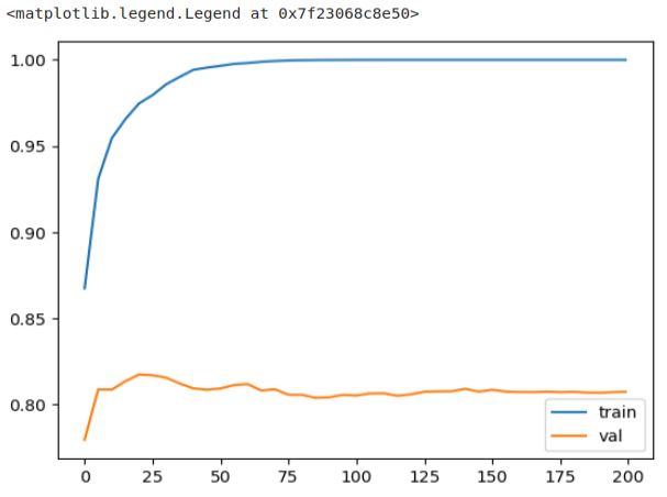
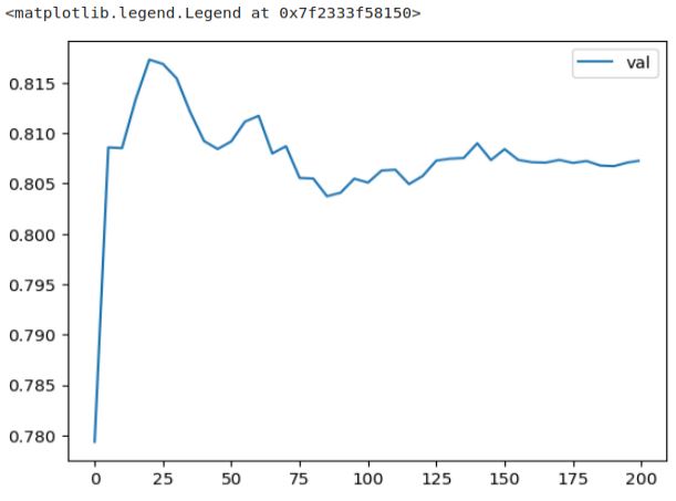
We can observe that the AUC on the training dataset consistently improves. However, the picture is different for the validation dataset. The curve reaches its peak earlier and then starts to decline and stagnate, indicating the onset of overfitting. This decline in performance on the validation dataset is more apparent when plotting only the AUC on validation, while the AUC on the training dataset remains consistently high. The decline in performance is more evident when we exclusively plot the validation graph.
plt.plot(df_score.num_iter, df_score.val_auc, label='val')
plt.legend()