
Ensemble and random forest
This article discusses the concept of Random Forest as a technique for combining multiple decision trees. Before diving into Random Forest, we’ll explore the concept of ensemble modeling, where multiple models act as a ‘board of experts.’ The final part of the article will cover the process of tuning a Random Forest model.
Board of experts
So far, we’ve been discussing the process when a client approaches a bank for a loan. They submit an application with basic information, and features are extracted from this application. These features are then fed into a decision tree, which provides a score representing the probability of the customer defaulting on the loan. Based on this score, the bank makes a lending decision.
Now, let’s imagine an alternative scenario where we don’t use a decision tree but rather rely on a ‘board of experts,’ consisting of five experts. When a customer submits an application, it’s distributed to each of these experts. Each expert independently evaluates the application and decides whether to approve or reject it. The final decision is determined by a majority vote—if the majority of experts say ‘yes,’ the bank approves the loan; if the majority says ‘no,’ the application is rejected.
The underlying concept of the ‘board of experts’ is based on the belief that the collective wisdom of five experts is more reliable than relying solely on one expert’s judgment. By aggregating multiple expert opinions, we aim to make better decisions.
This same concept can be applied to models. Instead of a ‘board of five experts,’ we can have five models (g1, g2, …, g5), each of which returns a probability of default. We can then aggregate these model predictions by calculating the average: (1/n) * Σ(pi).
Ensembling models
This method of aggregating multiple models is applicable to any type of model. However, in this case, we specifically focus on using decision trees. When we ensemble decision trees, we create what is known as a ‘random forest.’
But you might wonder, why do we call it a ‘random forest’ and not just a ‘forest’? The reason is that if we take the same application (with the same set of features) and build the same group of trees with identical parameters, the resulting trees would also be identical. These identical trees would produce exactly the same probability of default, and therefore, the average would be the same as well. Essentially, we would be training the same model five times, which is not what we want.
To avoid this redundancy and bring the ‘random’ element into play, a ‘random forest’ introduces variability during the training process by using bootstrapped samples and random subsets of features, leading to a more diverse and robust ensemble of decision trees.
Random forest – ensembling decision trees
So, what exactly happens in a random forest?
In a random forest, each of the applications or features that the trees receive is slightly different. For instance, if we have a total of 10 features, each tree might receive 7 out of the 10 features, creating a distinct set for each tree.
To illustrate this with a smaller example, let’s consider 3 features: assets, debt, and price. If we train only 3 models, we might have the following feature sets for each:
- Decision Tree #1: Features – assets, debt
- Decision Tree #2: Features – assets, price
- Decision Tree #3: Features – debt, price
This way, we have 3 different models. To obtain the final prediction, we calculate the average score as (1/3) * (p1 + p2 + p3). While in this simplified example, the feature selection is not entirely random due to the limited number of features, the real idea is to select features randomly from a larger set.
In a random forest, each model gets a random subset of features, and the response generated by the ensemble will be a probability of default. This is the fundamental concept behind a random forest. To use it in scikit-learn, you need to import it from the ensemble package.
from sklearn.ensemble import RandomForestClassifier

# n_estimators - number of models we want to use
rf = RandomForestClassifier(n_estimators=10)
rf.fit(X_train, y_train)

y_pred = rf.predict_proba(X_val)[:, 1]
roc_auc_score(y_val, y_pred)
# Output: 0.781835024581628

rf.predict_proba(X_val[[0]])
# Output: array([[1., 0.]])
This model achieves an AUC score of 78.2%, which is relatively good. Notably, this performance is on par with the best decision tree model without any specific tuning. In this instance, we used the default hyperparameters and only reduced the ‘n_estimators’ value from the default of 100 to 10.
However, it’s important to recognize that a random forest introduces an element of randomness during training. Consequently, when we retrain the model and make predictions again, we may obtain slightly different results due to this randomization. To ensure consistent and reproducible results, we can use the ‘random_state’ parameter. By setting a fixed ‘random_state,’ regardless of how many times we run the model, the results will remain the same.
rf = RandomForestClassifier(n_estimators=10, random_state=1)
rf.fit(X_train, y_train)

y_pred = rf.predict_proba(X_val)[:, 1]
roc_auc_score(y_val, y_pred)
# Output: 0.7744726453706618

rf.predict_proba(X_val[[0]])
# Output: array([[0.9, 0.1]])
Tuning random forest
Let’s delve into the possibilities of fine-tuning our random forest model. To start, we’ll explore how the model’s performance evolves when we increase the number of estimators or models it employs. Our approach will involve iterating over a range of values to observe how the model’s performance improves or changes with an increasing number of trees.
scores = []

for n in range(10, 201, 10):
    rf = RandomForestClassifier(n_estimators=n, random_state=1)
    rf.fit(X_train, y_train)

    y_pred = rf.predict_proba(X_val)[:, 1]
    auc = roc_auc_score(y_val, y_pred)

    scores.append((n, auc))

df_scores = pd.DataFrame(scores, columns=['n_estimators', 'auc'])
df_scores
| n_estimators | auc | |
|---|---|---|
| 0 | 10 | 0.774473 |
| 1 | 20 | 0.803532 |
| 2 | 30 | 0.815075 |
| 3 | 40 | 0.815686 |
| 4 | 50 | 0.817082 |
| 5 | 60 | 0.816458 |
| 6 | 70 | 0.817321 |
| 7 | 80 | 0.816307 |
| 8 | 90 | 0.816824 |
| 9 | 100 | 0.817599 |
| 10 | 110 | 0.817527 |
| 11 | 120 | 0.817939 |
| 12 | 130 | 0.818253 |
| 13 | 140 | 0.818102 |
| 14 | 150 | 0.817270 |
| 15 | 160 | 0.817981 |
| 16 | 170 | 0.817606 |
| 17 | 180 | 0.817463 |
| 18 | 190 | 0.817981 |
| 19 | 200 | 0.819050 |
# x-axis - n_estimators
# y-axis - auc score
plt.plot(df_scores.n_estimators, df_scores.auc)
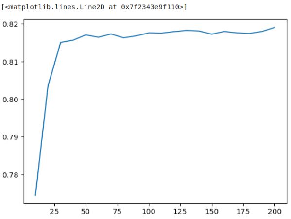
We observe that the model’s performance improves as we increase the number of estimators up to 50, but beyond that point, it reaches a plateau. Additional trees don’t significantly enhance the performance. Hence, training more than 50 trees doesn’t appear to be beneficial.
Now, let’s proceed with tuning our random forest model. It’s important to note that a random forest comprises multiple decision trees, so the parameters we tune within the random forest are essentially the same—specifically, we are interested in the max_depth and min_samples_leaf parameters. Starting with the max_dept‘ parameter, we aim to train a random forest model with different depth values to assess its impact on performance.
scores = []

for d in [5, 10, 15]:
    for n in range(10, 201, 10):
        rf = RandomForestClassifier(n_estimators=n,
                                    max_depth=d,
                                    random_state=1)
        rf.fit(X_train, y_train)

        y_pred = rf.predict_proba(X_val)[:, 1]
        auc = roc_auc_score(y_val, y_pred)

        scores.append((d, n, auc))

columns = ['max_depth', 'n_estimators', 'auc']
df_scores = pd.DataFrame(scores, columns=columns)
df_scores.head()
| max_depth | n_estimators | auc | |
|---|---|---|---|
| 0 | 5 | 10 | 0.787699 |
| 1 | 5 | 20 | 0.797731 |
| 2 | 5 | 30 | 0.800305 |
| 3 | 5 | 40 | 0.799708 |
| 4 | 5 | 50 | 0.799878 |
# Let's plot it
for d in [5, 10, 15]:
    df_subset = df_scores[df_scores.max_depth == d]

    plt.plot(df_subset.n_estimators, df_subset.auc,
             label='max_depth=%d' % d)

plt.legend()
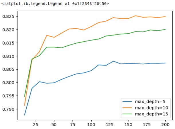
In the plot, we can observe that the AUC scores for ‘max_depth’ values of 10 and 15 are initially quite close, but after a certain point, the score for ‘max_depth‘ 15 begins to level off, showing only marginal improvement. In contrast, ‘max_depth‘ 10 continues to perform significantly better, peaking at around 125. This clearly illustrates that the choice of ‘max_depth‘ indeed matters. We can confidently select a value of 10 as the best choice, as the difference between 10 and 15, and between 10 and 5, is notably significant.
# Let's select 10 as the best value
max_depth = 10
Now, we’ll proceed to find the optimal value for the ‘min_samples_leaf’ parameter using a similar method as before.
scores = []

for s in [1, 3, 5, 10, 50]:
    for n in range(10, 201, 10):
        rf = RandomForestClassifier(n_estimators=n,
                                    max_depth=max_depth,
                                    min_samples_leaf=s,
                                    random_state=1)
        rf.fit(X_train, y_train)

        y_pred = rf.predict_proba(X_val)[:, 1]
        auc = roc_auc_score(y_val, y_pred)

        scores.append((s, n, auc))

columns = ['min_samples_leaf', 'n_estimators', 'auc']
df_scores = pd.DataFrame(scores, columns=columns)
For a better distinction between the graphs in the following plot we can change the colors as you see in the next two snippets.
colors = ['black', 'blue', 'orange', 'red', 'grey']
min_samples_leaf_values = [1, 3, 5, 10, 50]
list(zip(min_samples_leaf_values, colors))

# Output: [(1, 'black'), (3, 'blue'), (5, 'orange'), (10, 'red'), (50, 'grey')]
colors = ['black', 'blue', 'orange', 'red', 'grey']
min_samples_leaf_values = [1, 3, 5, 10, 50]

for s, col in zip(min_samples_leaf_values, colors):
    df_subset = df_scores[df_scores.min_samples_leaf == s]

    plt.plot(df_subset.n_estimators, df_subset.auc,
             color=col,
             label='min_samples_leaf=%d' % s)

plt.legend()
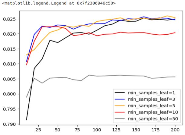
We can observe that ‘min_samples_leaf’ set to 50 performs the worst, while the three most favorable options are 1, 3, and 5. Among these, ‘min_samples_leaf’ of 3 stands out a good choice since it achieves good performance earlier than the others.
# Let's select 3 as the best value
min_samples_leaf = 3
Now, we’re ready to retrain the model using these selected values.
rf = RandomForestClassifier(n_estimators=100,
                            max_depth=max_depth,
                            min_samples_leaf=min_samples_leaf,
                            random_state=1,
                            n_jobs=-1)
rf.fit(X_train, y_train)

# Output:
# RandomForestClassifier(max_depth=10, min_samples_leaf=3, n_jobs=-1,
#                       random_state=1)
These are not the only two parameters we can tune in a random forest model. There are several other useful parameters to consider:
- max_features: This parameter determines how many features each decision tree receives during training. It’s essential to remember that random forests work by selecting only a subset of features for each tree.
- bootstrap: Bootstrap introduces another form of randomization, but at the row level. This randomization ensures that the decision trees are as diverse as possible.
- n_jobs: The training of decision trees can be parallelized because all the models are independent of each other. The ‘n_jobs’ parameter specifies how many trees can be trained in parallel. The default is ‘None,’ which means no parallelization. Using ‘-1’ means utilizing all available processors, which can significantly speed up the training process.”
These additional parameters offer opportunities for further fine-tuning and customization of your random forest model. For additional details and documentation on these parameters, you can refer to the official Scikit-Learn website.
