1. Accuracy and Dummy Model
   1. Evaluate the model on different thresholds
   2. Check Accuracy of Dummy Baseline

Accuracy and Dummy Model

In the last article, we calculated that our model achieved an accuracy of 80% on the validation data. Now, let’s determine whether this is a good value or not.

Accuracy measures the fraction of correct predictions made by the model.

In our evaluation, we checked each customer in the validation dataset to determine whether the model’s churn prediction was correct or incorrect. This decision was based on our threshold of 0.5, meaning a customer with a predicted value greater than or equal to 0.5 was considered a churning customer, while values below the threshold were considered non-churning customers.

Out of the 1409 customers in the validation dataset, we made 1132 correct predictions. Therefore, the accuracy is calculated as 1132/1409 = 0.80, which corresponds to 80%. This accuracy indicates that our model correctly predicted the churn status for 80% of the customers in the validation dataset. Whether this is considered good or not depends on the specific context and requirements of the problem.

len(y_val)
# Output: 1409

(y_val == churn_decision).sum()
# Output: 1132

1132 / 1409
# Output: 0.8034

(y_val == churn_decision).mean()
# Output: 0.8034

Evaluate the model on different thresholds

The question now is whether we have chosen a good value for the threshold. To evaluate this, we can adjust the threshold and perform validation again. By systematically varying the threshold, we can observe whether it improves the accuracy or not. To do this, we can use the ‘linspace’ function from NumPy to generate an array with multiple threshold values (e.g., 21 values evenly spaced between 0 and 1). For each threshold value, we can calculate the accuracy and then determine the best threshold value based on the validation results. This process allows us to fine-tune the threshold to optimize the model’s performance.

thresholds = np.linspace(0, 1, 21)
thresholds

# Output:        
# array([0.  , 0.05, 0.1 , 0.15, 0.2 , 0.25, 0.3 , 0.35, 0.4 , 0.45, 0.5 ,
#        0.55, 0.6 , 0.65, 0.7 , 0.75, 0.8 , 0.85, 0.9 , 0.95, 1.  ])

scores = []

for t in thresholds:
    churn_decision = (y_pred >= t)
    score = (y_val == churn_decision).mean()
    print('%.2f %.3f' % (t, score))
    scores.append(score)

# Output: 
# 0.00 0.274
# 0.05 0.509
# 0.10 0.591
# 0.15 0.666
# 0.20 0.710
# 0.25 0.739
# 0.30 0.760
# 0.35 0.772
# 0.40 0.785
# 0.45 0.793
# 0.50 0.803
# 0.55 0.801
# 0.60 0.795
# 0.65 0.786
# 0.70 0.766
# 0.75 0.744
# 0.80 0.735
# 0.85 0.726
# 0.90 0.726
# 0.95 0.726
# 1.00 0.726

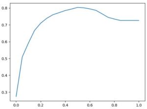
It appears that 0.5 is indeed the best threshold based on the validation set. This suggests that the default threshold of 0.5 is an appropriate choice for our model in this context. To visually represent this threshold optimization process, we can create a plot. The x-axis will represent the threshold values, while the y-axis will represent the corresponding scores (in this case, accuracy or another relevant metric). This plot will provide a clear visualization of how the model’s performance varies with different threshold values, helping us identify the threshold that maximizes the desired metric.

plt.plot(thresholds,scores)

While we used our custom function to calculate accuracy, it’s worth noting that Scikit-Learn provides built-in functions for common evaluation metrics, including accuracy. These built-in functions can simplify the process of evaluating your model’s performance, making it more convenient and efficient.

from sklearn.metrics import accuracy_score

thresholds = np.linspace(0, 1, 21)
scores = []

for t in thresholds:
    score = accuracy_score(y_val, y_pred >= t)
    print('%.2f %.3f' % (t, score))
    scores.append(score)

# Output: 
# 0.00 0.274
# 0.05 0.509
# 0.10 0.591
# 0.15 0.666
# 0.20 0.710
# 0.25 0.739
# 0.30 0.760
# 0.35 0.772
# 0.40 0.785
# 0.45 0.793
# 0.50 0.803
# 0.55 0.801
# 0.60 0.795
# 0.65 0.786
# 0.70 0.766
# 0.75 0.744
# 0.80 0.735
# 0.85 0.726
# 0.90 0.726
# 0.95 0.726
# 1.00 0.726

Check Accuracy of Dummy Baseline

There is an important point about the limitations of accuracy as an evaluation metric. While we may achieve a certain level of accuracy, it doesn’t always provide the full picture of a model’s performance, especially in cases with imbalanced datasets or when specific types of errors are more critical than others.

In this example, I’ve mentioned that the accuracy of the model is 80%, but a dummy model that predicts all customers as not churning achieves an accuracy of 73%. This highlights the issue with accuracy, as it doesn’t differentiate between different types of errors. In churn prediction, false negatives (predicting a customer won’t churn when they actually do) can be more costly than false positives (predicting a customer will churn when they won’t).

Choosing the most appropriate evaluation metric depends on the specific goals and requirements of the problem. For example, in cases where minimizing false negatives is crucial (e.g., in medical diagnoses or fraud detection), recall may be a more relevant metric than accuracy.

from collections import Counter

Counter(y_pred >= 1.0)
# Output: Counter({False: 1409})

# Distribution of y_val
Counter(y_val)

# Output: Counter({0: 1023, 1: 386})

1023 / 1409
# Output: 0.7260468417317246

y_val.mean()
# Output: 0.2739531582682754

1 - y_val.mean()
# Output: 0.7260468417317246

We can observe that there are significantly more non-churning customers than churning ones, with only 27% being churning customers and 73% being non-churning customers. This situation highlights a common challenge known as class imbalance, where one class has far more samples than the other.

In cases of class imbalance, the traditional accuracy metric can be misleading. For example, a dummy model that predicts the majority class for all samples can achieve a high accuracy simply by getting most of the samples right for the majority class. However, it will perform poorly in identifying the minority class (in this case, the churning customers), which is often more crucial to predict accurately.

To effectively address class imbalance and evaluate our model, we should consider alternative metrics such as:

1. Precision: This metric measures the proportion of true positive predictions among all positive predictions. It is particularly useful when the cost of false positives is high.
2. Recall: Recall measures the proportion of true positive predictions among all actual positive instances. It is valuable when the cost of false negatives is significant.
3. F1-Score: The F1-Score is the harmonic mean of precision and recall, providing a balanced measure that considers both false positives and false negatives.
4. Area Under the Receiver Operating Characteristic Curve (AUC-ROC): The ROC curve plots the true positive rate against the false positive rate at various threshold settings. The AUC-ROC score assesses the classifier’s ability to distinguish between the positive and negative classes, making it particularly useful for imbalanced datasets.

Selecting the appropriate evaluation metric depends on the specific goals and requirements of the problem. In cases of class imbalance, accurate identification of the minority class (churning customers) is crucial.