
Logistic Regression
As mentioned earlier, classification problems can be categorized into binary problems and multi-class problems. Binary problems are the types of problems that logistic regression is typically used to solve.
In binary classification, the target variable yiyi belongs to one of two classes: 0 or 1. These classes are often referred to as “negative” and “positive,” and they represent two mutually exclusive outcomes. In the context of churn prediction, “no churn” and “churn” are examples of binary classes. Similarly, in email classification, “no spam” and “spam” are also binary classes.
That means g(xi) outputs a number from 0 to 1 that we can treat as the probability of xi belonging to the positive class.
Formula:
Linear regression: g(xi)=w0+wTxi → outputs a number −∞..∞∈R
- x0 – bias term
- wT – weights vector
- xi – features
Logistic regression: g(xi)=SIGMOID(w0+wTxi) → outputs a number 0..1∈R
sigmoid(z)= 1 / (1+exp(−z))
This function maps any real number z to the range of 0 to 1, making it suitable for modeling probabilities in logistic regression. We’ll use this function to convert a score into a probability.
Let’s see how to implement the sigmoid function and use it. We can create an array with 51 values between -7 and 7 using np.linspace(-7, 7, 51). This is our z in the next snippet.
def sigmoid(z):
    return 1 / (1 + np.exp(-z))

z = np.linspace(-7, 7, 51)
z
# Output:
# array([-7.0000000e+00, -6.7200000e+00, -6.4400000e+00, -6.1600000e+00,
#       -5.8800000e+00, -5.6000000e+00, -5.3200000e+00, -5.0400000e+00,
#       -4.7600000e+00, -4.4800000e+00, -4.2000000e+00, -3.9200000e+00,
#       -3.6400000e+00, -3.3600000e+00, -3.0800000e+00, -2.8000000e+00,
#       -2.5200000e+00, -2.2400000e+00, -1.9600000e+00, -1.6800000e+00,
#       -1.4000000e+00, -1.1200000e+00, -8.4000000e-01, -5.6000000e-01,
#       -2.8000000e-01,  8.8817842e-16,  2.8000000e-01,  5.6000000e-01,
#        8.4000000e-01,  1.1200000e+00,  1.4000000e+00,  1.6800000e+00,
#        1.9600000e+00,  2.2400000e+00,  2.5200000e+00,  2.8000000e+00,
#        3.0800000e+00,  3.3600000e+00,  3.6400000e+00,  3.9200000e+00,
#        4.2000000e+00,  4.4800000e+00,  4.7600000e+00,  5.0400000e+00,
#        5.3200000e+00,  5.6000000e+00,  5.8800000e+00,  6.1600000e+00,
#        6.4400000e+00,  6.7200000e+00,  7.0000000e+00])
We can apply this sigmoid function to our array z,…
sigmoid(z)

# Output:
# array([9.11051194e-04, 1.20508423e-03, 1.59386223e-03, 2.10780106e-03,
#             2.78699622e-03, 3.68423990e-03, 4.86893124e-03, 6.43210847e-03,
#             8.49286285e-03, 1.12064063e-02, 1.47740317e-02, 1.94550846e-02,
#             2.55807883e-02, 3.35692233e-02, 4.39398154e-02, 5.73241759e-02,
#             7.44679452e-02, 9.62155417e-02, 1.23467048e-01, 1.57095469e-01,
#             1.97816111e-01, 2.46011284e-01, 3.01534784e-01, 3.63547460e-01,
#             4.30453776e-01, 5.00000000e-01, 5.69546224e-01, 6.36452540e-01,
#             6.98465216e-01, 7.53988716e-01, 8.02183889e-01, 8.42904531e-01,
#             8.76532952e-01, 9.03784458e-01, 9.25532055e-01, 9.42675824e-01,
#             9.56060185e-01, 9.66430777e-01, 9.74419212e-01, 9.80544915e-01,
#             9.85225968e-01, 9.88793594e-01, 9.91507137e-01, 9.93567892e-01,
#             9.95131069e-01, 9.96315760e-01, 9.97213004e-01, 9.97892199e-01,
#             9.98406138e-01, 9.98794916e-01, 9.99088949e-01])
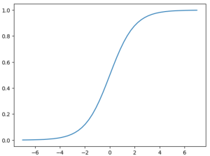
… but let’s visualize how the graph of the sigmoid function looks.
plt.plot(z, sigmoid(z))
At the end of this article, both implementations are presented for comparison. The first snippet demonstrates the familiar linear regression, while the second snippet illustrates logistic regression. It’s evident that there is essentially only one difference between the two: in logistic regression, the sigmoid function is applied to the result of the linear regression to transform it into a probability value between 0 and 1.
def linear_regression(xi):
    result = w0

    for j in range(len(w)):
        result = result + xi[j] * w[j]

    return result
def logistic_regression(xi):
    score = w0

    for j in range(len(w)):
        score = score + xi[j] * w[j]

    result = sigmoid(score)
    return result
Linear regression and logistic regression are called linear models, because dot product in linear algebra is a linear operator. Linear models are fast to use, fast to train.
