
Simple feature engineering
Suppose we want to develop a new feature based on the existing ones in the feature matrix X. Let’s assume we want to use the year information as an age information. Let’s assume further we have year 2017.
2017 - df_train.year
# Output:
# 0        8
# 1        1
# 2       22
# 3        1
# 4        3
#         ..
# 7145     1
# 7146    10
# 7147     6
# 7148     3
# 7149    19
# Name: year, Length: 7150, dtype: int64
We can add this new feature ‘age’ to our prepare_X function. What is one important remark here. It’s a good way to copy the dataframe inside prepare_X. Otherwise while using df you’ll modify the original data, what ist mostly not wanted.
base = ['engine_hp', 'engine_cylinders', 'highway_mpg', 'city_mpg', 'popularity']

def prepare_X(df):
    df = df.copy()

    df['age'] = 2017 - df.year
    features = base + ['age']

    df_num = df[features]
    df_num = df_num.fillna(0)
    # extracting the Numpy array
    X = df_num.values
    return X

X_train = prepare_X(df_train)
X_train
# Output:
# array([[3.100e+02, 8.000e+00, 1.800e+01, 1.300e+01, 1.851e+03, 8.000e+00],
#       [1.700e+02, 4.000e+00, 3.200e+01, 2.400e+01, 6.400e+02, 1.000e+00],
#       [1.650e+02, 6.000e+00, 1.500e+01, 1.300e+01, 5.490e+02, 2.200e+01],
#       ...,
#       [3.420e+02, 8.000e+00, 2.400e+01, 1.700e+01, 4.540e+02, 6.000e+00],
#       [1.700e+02, 4.000e+00, 2.800e+01, 2.300e+01, 2.009e+03, 3.000e+00],
#       [1.600e+02, 6.000e+00, 1.900e+01, 1.400e+01, 5.860e+02, 1.900e+01]])
The output of the last snippet shows a list of lists. Each list has 6 items – 5 numerical columns and our new ‘age’ column. Let’s train a new model and see how the model performs.
X_train = prepare_X(df_train)
w0, w = train_linear_regression(X_train, y_train)

X_val = prepare_X(df_val)
y_pred = w0 + X_val.dot(w)

rmse(y_val, y_pred)
# Output: 0.5153662333982238
We can see an improvement. The rmse decreased from 0.7328022115111966 to 0.5153662333982238. The improvement in the rmse was clear. Let’s see if this improvement can be seen in the plots as well.
sns.histplot(y_pred, color='red', alpha=0.5, bins=50)
sns.histplot(y_val, color='blue', alpha=0.5, bins=50)
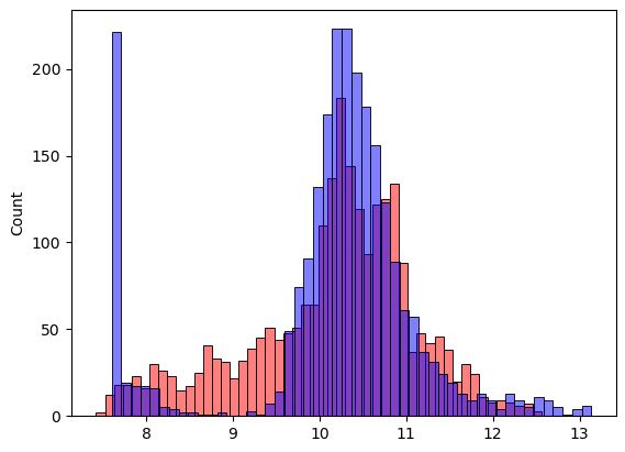
Here, too, a clear improvement can be seen. Many car prices are predicted much better. But there is still space for improvement.
