
This part is about RMSE as an objective way to evaluate the model performance. In the first part of this article RMSE is introduced and in the second part RMSE is used to evaluate our model on unseen data.
Root Mean Squared Error – RMSE
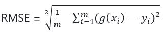
We have the following variables, so we can calculate the RMSE.
- g(xi) – prediction for xi (observation i)
- yi – actual value
- m – number of different observations
- –> g(xi) – yi is the difference between the prediction and the actual value
First let’s look at this with an simplified example. First step is to calculate the difference between the prediction and the actual values.
| y_pred | 10 | 9 | 11 | … | 10 |
| y_train | 9 | 9 | 10.5 | … | 11.5 |
| y_pred – y_train | 1 | 0 | 0.5 | … | -1.5 |
Then we need to square this difference to get the squared error.
| square the difference: (g(xi) – yi)² | 1 | 0 | 0.25 | … | 2.25 | SQUARED ERROR |
Then we divide the squared error by number of observations to get the mean squared error. Lastly we can calculate the root mean squared error and we’re done.
| average | (1 + 0 + 0.25 + 2.25) / 4 = 0.875 | MEAN SQUARED ERROR |
| root | sqrt(0.875) = 0.93 | ROOT MEAN SQUARED ERROR |
We can implement the RMSE in code. This could look like:
def rmse(y, y_pred):
    se = (y - y_pred) ** 2
    mse = se.mean()
    return np.sqrt(mse)
In the last article we used Seaborn to visualize the performance but now we have an objective metric for the evaluation.
rmse(y_train, y_pred)
# Output: 0.7464137917148924
Validating the model
Evaluating the model performance on the training data does not really give a good indication of the real model performance. Since we don’t know how well the model can apply the learned knowledge to unseen data. So what we want to do now after training the model g on our training dataset, we want to apply it on the validation dataset to see how it performs on unseen data. We use RMSE for validating the performance.
base = ['engine_hp', 'engine_cylinders', 'highway_mpg', 'city_mpg', 'popularity']

X_train = df_train[base].fillna(0).values

w0, w = train_linear_regression(X_train, y_train)

y_pred = w0 + X_train.dot(w)
Next we implement the prepare_X function. The idea here to provide the same way of preparing the dataset regardless of whether it’s train set, validation set, or test set.
def prepare_X(df):
    df_num = df[base]
    df_num = df_num.fillna(0)
    # extracting the Numpy array
    X = df_num.values
    return X
Now we can use this function when we prepare data for the training and for the validation as well. In the training part we only use training dataset to train the model. In the validation part we prepare the validation dataset the same way like before and apply the model. Lastly we compute the rmse.
# Training part:
X_train = prepare_X(df_train)
w0, w = train_linear_regression(X_train, y_train)

# Validation part:
X_val = prepare_X(df_val)
y_pred = w0 + X_val.dot(w)

# Evaluation part:
rmse(y_val, y_pred)
# Output: 0.7328022115111966
When we compare the RMSE from training with the value from validation (0.746 vs. 0.733) we see that the model performs similarly well on the seen and unseen data. That is what we have hoped for.
