Linear regression vector form

This article covers the generalization to a vector form of what we did in the last article. That means coming back from only one observation x_i (of one car) to the whole feature matrix X.

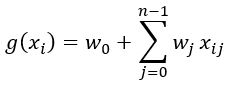
Looking at the last part of this formula we see the dot product (vector-vector multiplication). g(x_i) = w0 + x_i^Tw

Let’s implement again the dot product (vector-vector multiplication)

def dot(xi, w):
    n = len(xi)
    
    res = 0.0
    for j in range(n):
        res = res + xi[j] * w[j]
        
    return res

Based on that the implementation of the linear_regression function could look like:

def linear_regression(xi):
    return w0 + dot(xi, w) 

To make the last equation more simple, we can imagine there is one more feature x_i0, that is always equal to 1.

g(x_i) = w₀ + x_i^Tw -> g(x_i) = w₀x_i0 + x_i^Tw

That means vector w becomes a n+1 dimensional vector:

• w = [w₀, w₁, w₂, … w_n]
• x_i = [x_i0, x_i1, x_i2, …, x_in] = [1, x_i1, x_i2, …, x_in]
• w^Tx_i = x_i^Tw = w₀ + …

That means we can use the dot product for the entire regression.

xi = [138, 24, 1385]
w0 = 7.17
w = [0.01, 0.04, 0.002]

# adding w0 to the vector w
w_new = [w0] + w
w_new
# Output: [7.17, 0.01, 0.04, 0.002]

xi
# Output: [138, 24, 1385]

The updated code for linear_regression function looks now like

def linear_regression(xi):
    xi = [1] + xi
    return dot(xi, w_new)

linear_regression(xi)
# Output: 12.280000000000001

Having done this, let’s go back to thinking about all the examples together.
X is a m x (n+1) dimensional matrix (with m rows and n+1 columns)

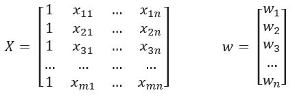
What we have to do here, for each row of X we multiply this row with the vector w. This vector contains our predictions, therefor we call it y_pred.

To sum up. What we need to do to get our model g is a matrix vector multiplication between X and w.

w0 = 7.17
w = [0.01, 0.04, 0.002]
w_new = [w0] + w

x1  = [1, 148, 24, 1385]
x2  = [1, 132, 25, 2031]
x10 = [1, 453, 11, 86]

# X becomes a list of lists
X = [x1, x2, x10]
X
# Output: [[1, 148, 24, 1385], [1, 132, 25, 2031], [1, 453, 11, 86]]

# This turns the list of lists into a matrix
X = np.array(X)
X
# Output:
# array([[   1,  148,   24, 1385],
#              [   1,  132,   25, 2031],
#              [   1,  453,   11,   86]])

# Now we have predictions, so for each car we have a price for this car
y = X.dot(w_new)

# shortcut to not do -1 manually to get the real $ price
np.expm1(y) 
# Output: array([237992.82334859, 768348.51018973, 222347.22211011])

The next snippet shows the implementation of the adapted linear_regression function

def linear_regression(X):
    return X.dot(w_new)

y = linear_regression(X)
np.expm1(y) 
# Output: array([237992.82334859, 768348.51018973, 222347.22211011])

Maybe you wonder where the w_new vector comes from. That’s the topic of the next article.