1. Linear regression
   1. Step back and focus on one observation
   2. Implementation of linear regression function

Linear regression

Let’s delve deeper into the topic of linear regression.

Linear regression is a fundamental statistical technique used in the field of machine learning for solving regression problems. In simple terms, regression analysis involves predicting a continuous outcome variable based on one or more input features. That means the output of the model is a number.

In the case of linear regression, the basic idea is to find the best-fitting linear relationship between the input features and the output variable. This relationship is represented by a linear equation of the form:

y = w₀ + w₁x₁ + w₂x₂ + … + w_nx_n

Here, “y” represents the output variable, and x₁, x₂, …, x_n represent the input features. The w₀, w₁, w₂, …, w_n are the coefficients that determine the relationship between the input features and the output variable.

The goal of linear regression is to estimate the values of these coefficients in such a way that the sum of squared differences between the observed and predicted values is minimized. This minimization is typically achieved using a method called “ordinary least squares,” which calculates the best-fitting line by minimizing the sum of the squared errors between the predicted and actual values.

Linear regression is widely used in various fields, including economics, finance, social sciences, and engineering, to name just a few. It provides a simple and interpretable way to understand the relationship between the input features and the continuous outcome variable.

In summary, linear regression is a powerful tool for predicting numerical values based on input features. By finding the best-fitting linear equation, it enables us to make accurate predictions and gain insights into the relationship between variables.

Step back and focus on one observation

Just to recap what we know from the articles before, there is the function g(X) ~ y with: g as the model (in our example Linear regression), X as the feature matrix and y as the target (in our example price).

Now let’s step back and look at only one observation. The corresponding function is g(x_i) ~ y_i with: x_i as one car and y_i as its price. So x_i is one specific row of the feature matrix X. We can think of it as a vector with multiple elements (n different characteristics of this one car).

x_i = (x_i1, x_i2, x_in) -> g(x_i1, x_i2, x_in) ~ y_i

Let’s look at one example and how this looks in code.

df_train.iloc[10]

# Output: 
# make                         chevrolet
# model                            sonic
# year                              2017
# engine_fuel_type      regular_unleaded
# engine_hp                        138.0
# engine_cylinders                   4.0
# transmission_type            automatic
# driven_wheels        front_wheel_drive
# number_of_doors                    4.0
# market_category                    NaN
# vehicle_size                   compact
# vehicle_style                    sedan
# highway_mpg                         34
# city_mpg                            24
# popularity                        1385
# Name: 10, dtype: object

We take as an example the characteristic enging_hp, city_mpg, and popularity.

xi = [138, 24, 1385]

That’s almost everything we need to implement g(x_i) ~ y_i:

• x_i = (138, 24, 1385)
• with i = 10
• need to implement the function g(x_i2,x_i2, … , x_in) ~ y_i

# in code this would look like --> this is what we want to implement

def g(xi):
    # do something and return the predicted price
    return 10000

g(xi)
# Output: 10000

However, this function g is still not very useful, because it always returns a fixed price. We need to implement the function

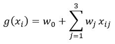
g(x_i) = w₀ + w₁x_i1 + w₂x_i2 + w₃x_i3

with w₀ as bias term and w₁, w₂, and w₃ as weights. This formula can be written as

Implementation of linear regression function

In general and because of array implementation in Python (indices of arrays start with 0 instead of 1), the formula for linear regression looks like this:

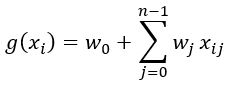
The following snippet shows the implementation of the g-function (renamed as linear_regression).

def linear_regression(xi):
    n = len(xi)    
    pred = w0
    
    for j in range(n):
        pred = pred + w[j] * xi[j]
    
    return pred

# sample values for w0 and w and the given xi
xi = [138, 24, 1385]
w0 = 0
w = [1, 1, 1]

linear_regression(xi)
# Output: 1547

# try some other values
w0 = 7.17
w = [0.01, 0.04, 0.002]
linear_regression(xi)
# Output: 12.280000000000001

What does this actually mean?

We’ve just implemented the formula as mentioned before with given values:
7.17 + 138*0.01 + 24*0.04 + 1385*0.002 = 12.28

• w₀ = 7.17 bias term = the prediction of a car, if we don’t know anything about this
• engine_hp: 138 * 0.01 that means in this case per 100 hp the price will increase by $1
• city_mpg: 24 * 0.04 that means analog to hp, the more gallons the higher the price will be
• popularity: 1385 * 0.002 analog, but it doesn’t seem that it’s affecting the price too much, so for every extra mention on twitter the car becomes just a little bit more expensive

There is still one important step to do. Because we logarithmized (log(y+1)) the price at the beginning, we now have to undo that. This gives us the predicted price in $. Our car has a price of $215,344.72.

# Get the real prediction for the price in $
# We do "-1" here to undo the "+1" inside the log
np.exp(12.280000000000001) - 1
# Output: 215344.7166272456

# Shortcut to not do -1 manually
np.expm1(12.280000000000001) 
# Output: 215344.7166272456

# Just for checking only
np.log1p(215344.7166272456)
# Output: 12.280000000000001